Operating Systems and System Software

Betriebssysteme und Systemsoftware

Prof. Redha Gouicem

Course Information

Overview

Who are we?

  • LuFG Betriebssysteme/Operating Systems
  • Teaching
  • Research


Betriebssysteme und Systemsoftware

  • Organisation
  • Evaluation
  • Links

Who Are We?

Lehr- und Forschungsgebiet Betriebssysteme
Operating Systems Research and Teaching Unit


Faculty

  • Prof. Redha Gouicem

Administration

  • Claudia Graf

Researchers

  • Jérôme Coquisart, M.Sc.
  • Mostafa Hadizadeh, M.Sc.

Research assistants - Tutors (HiWi)

  • 16 people, both bachelor and master students

Where Can You Find Us?

Our offices are in the UMIC building, 2nd floor

Teaching Curriculum

Research Activities

As the name of the group suggests, operating systems!

In short: design, implementation and optimisation of the lower software stack, between the hardware and users.

The main goals are:

  • Enable users to have an efficient and reliable execution environment for their applications,
  • Allow developers to have an easy-to-use abstraction of the hardware and transparent resource management and isolation

We will see in this course what an operating system is in more details!


In a nutshell, our topics revolve around:


“Classical” operating systems

  • Scheduling
  • Memory management
  • Storage systems
  • Unikernels

Virtualisation

  • Hypervisors
  • Containers
  • Deployment models

Emerging hardware

  • Non-volatile memory
  • FPGAs
  • CXL

Binary translation

  • Cross architecture emulators
  • Memory models
  • Correctness

Operating Systems and System Software: Team

Lecturer:

Prof. Redha Gouicem


Teaching assistants:

  • Mostafa Hadizadeh, M.Sc.
  • Justus Breyer, M.Sc. (COMSYS)


Tutors:

  • Ansarinia Alireza
  • Fehrenbacher Marvin
  • Giese Cedrick
  • Klinkmann Lasse
  • Lu Cheng-Yo
  • May Luca
  • Schmitt Lukas
  • Szymanski Oskar
  • Tugsbayar Jan
  • Bahkan Anas
  • Schröder Janik Felix
  • Slowikowska Natalia
  • Fehr Henric
  • Richi Omar
  • Dierker Felix

Contact emails

Organisation

  • Lectures: 2x week, 1.5 hours each
  • Exercises: 1x week
    Present solutions to the previous week’s assignments
  • Tutorials: 1x week, 20 groups (EN, DE or both)
    Solve and discuss assignments in small groups


Topics:

  • Introduction to operating systems
  • Processes and threads / Scheduling
  • Memory management
  • File management
  • I/O devices and interrupts
  • Concurrency and Synchronization
  • User space OS (System calls, shared libraries)
  • Virtualization and containers

Week Planning

Day Time Where Room
Lectures Monday 16:30 – 18:00 1385 C.A.R.L. 102
Tuesday 14:30 – 16:00 1385 C.A.R.L. 102
Exercise Thursday 14:30 – 16:00 1515 TEMP 002


Tutorial groups:

Monday Tuesday Wednesday Thursday Friday
08:30 - 10:00 7, 19 10 2, 22 4, 15
10:30 - 12:00 14 8
12:30 - 14:00 6, 21 1, 17 9, 16 24
14:30 - 16:00 Lecture 3, 12 Global exercise 11, 18
16:30 - 18:00 Lecture 5, 23 13, 25

Check slots and register on RWTHonline!

Weekly Programming Assignments

Every week, you get programming assignments:

  • On Moodle, with the VPL platform
  • Automatically graded
  • Individual submission, but you are allowed to help each other in small groups (without copying solutions)


Planning:

For a given topic \(T_i\), e.g., memory management:

  • The tutorials covering \(T_i\) will happen on week \(i\)
  • After the last tutorial on week \(i\), the graded assignment will be released (Friday at around 16:30)
  • You have a week to complete the graded assignment, until the following Global Exercise (Thursday 14:30), on week \(T_{i+1}\)
    This gives you roughly 10-12 days to complete the assignment, depending on the week
  • The assignment solution will be provided and discussed in the Global Exercise just after the deadline (Thursday 14:30), on week \(T_{i+1}\)

The VPL platform will run tests on a Linux system.

If you want to work locally on your own machine (and not directly on Moodle), we strongly recommend using Linux.
You can also use Windows with the Windows Subsystem for Linux (WSL) or MacOS.

Course Evaluation

Weekly assignments

Programming assignments on VPL every week.
At the end of the semester, a special bonus assignment will be released.

Weight: 20% of the final grade + 10% bonus points for the exam


Written exam

Mostly concept questions and exercises. You won’t have to write code from scratch.
At most, we may give you some code to read and explain/fix, or have you write a couple of lines.

Weight: 80% of the final grade


You need to get a passing grade (half of the total points) in both to pass the course!

Course Survey

Please give us feedback on things that you disliked or feel could be improved, but also on the things that you liked!

This is very important for us, especially since this course has been heavily refactored.

We need your opinion to improve the course for future years!


You have until 09.07.2025 23:59:00 to fill in the evaluation forms.

Below, you can find two forms: one for the lecture where you can give us feedback about everything except tutorials, and one for the tutorials.


Lecture evaluation

Link

Tutorial evaluation

Link

For tutorials, please do not forget to specify the number of your tutorial group, or the name of your tutor!

References

Books

  • Modern Operating Systems, Fifth Edition
    Andrew S. Tanenbaum, Herbert Bos (2023)
  • The Design and Implementation of the FreeBSD Operating System, Second Edition
    Marshall K. McKusick, George V. Neville-Neil, Robert N.M. Watson (2015)
  • The C Programming Language, Second Edition
    Brian W. Kernighan, Dennis M. Ritchie (1988)
  • Linux Kernel Development, Third Edition
    Robert Love (2010)

Chapter 1: Introduction to Operating Systems

This Week’s Program

In this first week, we’ll start slow, first defining what an operating system is, its general architecture, and how it is used by applications.


  1. Overview of Operating Systems
    Definitions and general concepts, history
  2. Protection Domains and Processor Privilege Levels
    Software and hardware isolation mechanisms between the OS and user applications
  3. Operating System Architectures
    Main OS architectures and designs, their pros and cons

Overview of Operating Systems

What Is an Operating System?

Computer systems are complex machines with a large number of components:

  • Internal chips: processor(s), memory
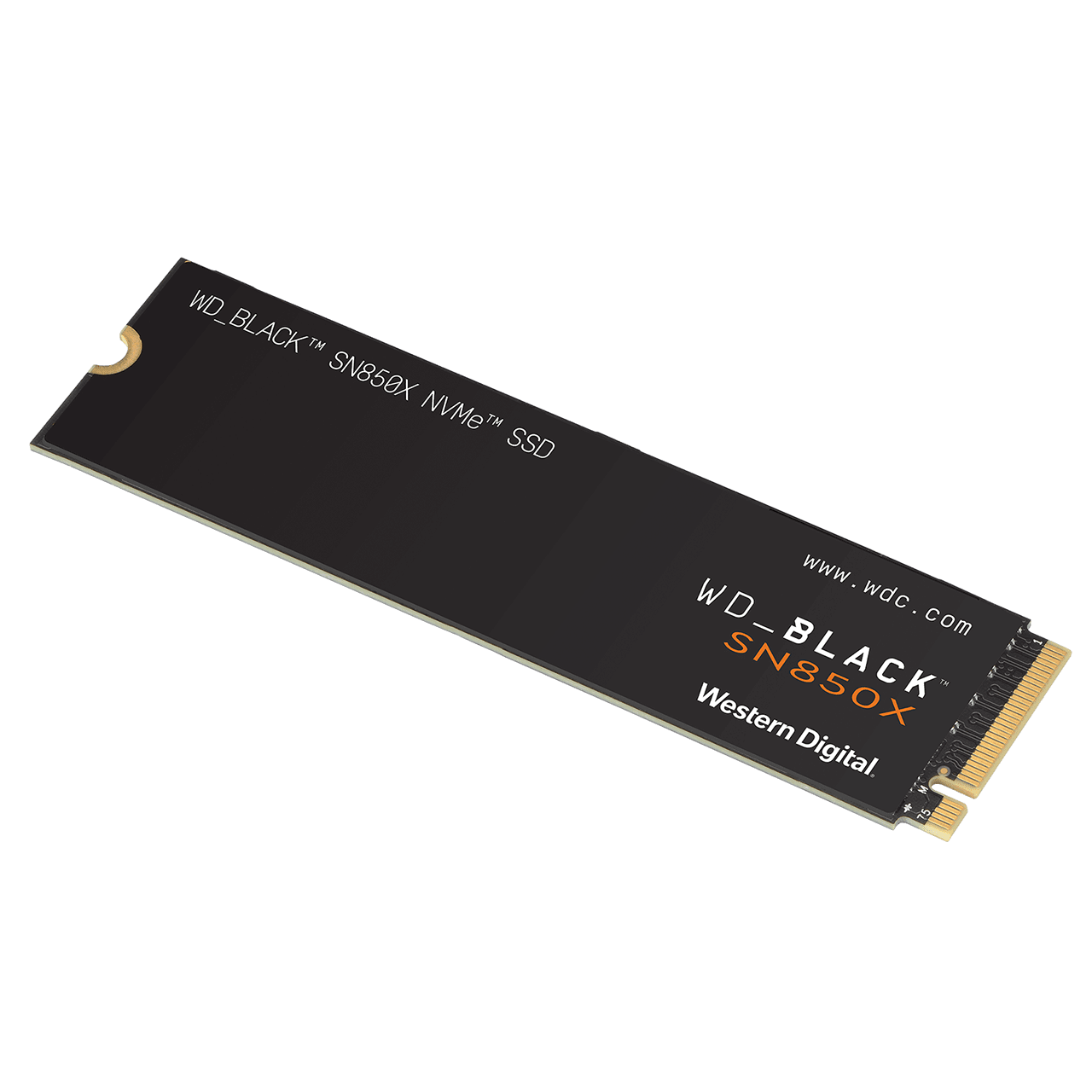
  • Storage devices: hard drives (HDD), solid state drives (SSD), etc.
  • PCI devices: network cards, graphics cards, etc.
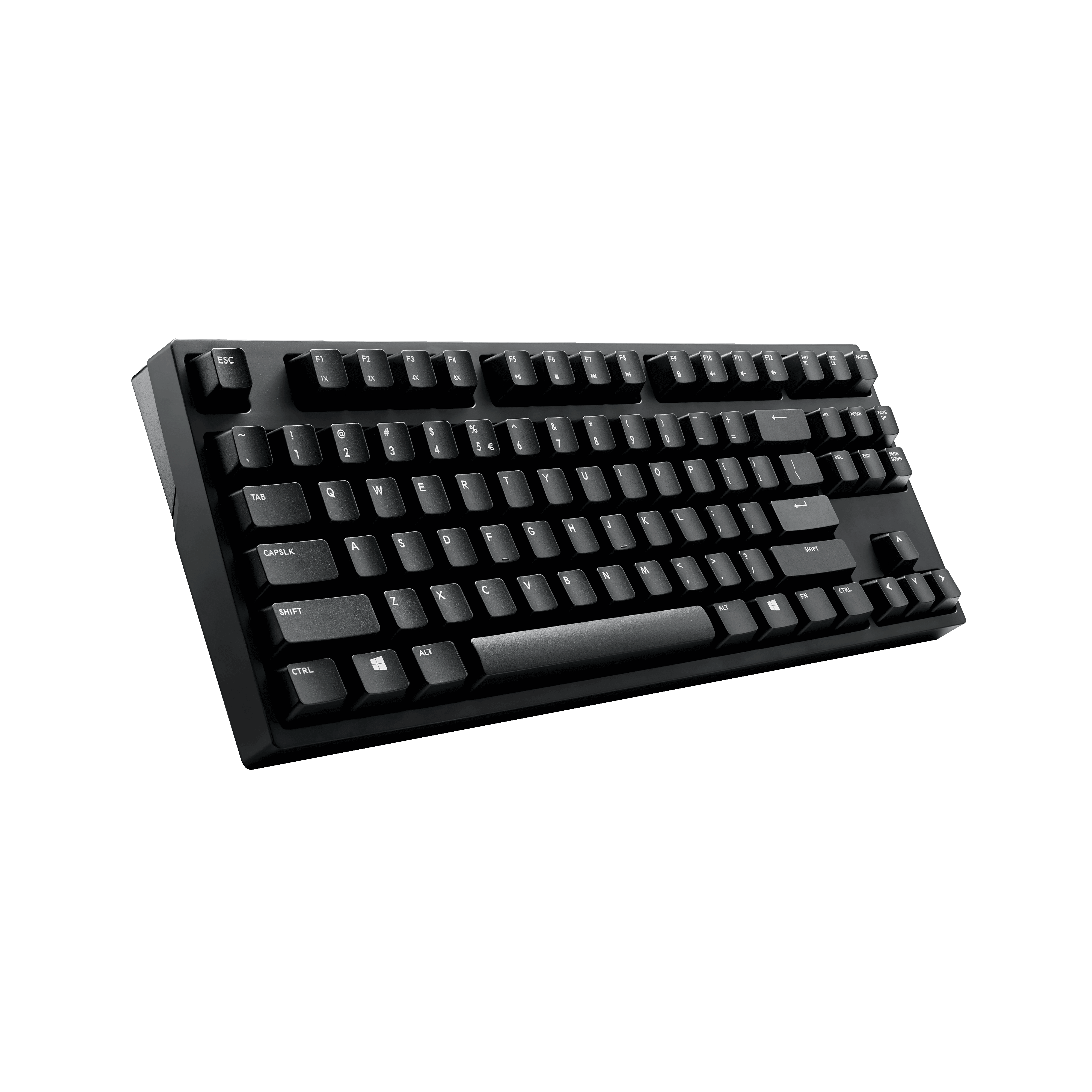
  • Peripherals: keyboard, mouse, display, etc.


Application programmers cannot be expected to know how to program all these devices.
And even if they do, they would rewrite the exact same code for every application,
e.g., the code to read inputs from the keyboard.


Resources can be shared by multiple programs.
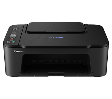
Expecting programs to collaborate and not mess with each other is not possible,
e.g., two programs try to print at the same time, but the printer can only print one coherent job at a time.


The operating system is the software layer that lies between applications and hardware.
It provides applications a simpler interface with hardware and manages resources.

What Is an Operating System? (2)

The operating system is the glue between hardware and user applications.

It can be split into two parts:

  • User interface programs: libraries, shell, graphical interfaces (GUI), etc.
    They offer a high level of abstractions, and are usually used by user applications to manipulate the underlying system.
  • Kernel: executes critical operations with a high level of privilege (supervisor mode) and directly interacts with hardware.
    User interface programs go through the kernel to manipulate the state of the underlying hardware.


In this course, we will mostly focus on the kernel part of the operating system.

What Is the Operating System’s Job?

The operating system has two main jobs:

  1. From the applications’ perspective: provide easy abstractions to use the hardware
  2. From the hardware’s perspective: manage the resources for controlled and safe use

Abstraction layer

Hardware is complex and provides messy interfaces. Devices may have their own design and interfaces, even when they have the same goal,
e.g., hard drives may respond to different types of commands for the same functional task.

Resource manager

Hardware resources are shared by multiple programs and need to be properly managed to allow safe use,
e.g., if two programs try to use the same hard drive, we need to make sure they are not unsafely modifying the same data.

The operating system must provide a simple and clean interface to access hardware resources.

The operating system must provide a safe and controlled allocation of resources to programs.

Main Operating System Services

Most operating systems are expected to provide the following features to user applications:

  1. Program management
    execution environment, synchronization, scheduling, etc.
  1. Memory management
    memory allocation, isolation
  1. File management
    file system, standardized API, cache, etc.
  1. Network management
    network topology, protocols, APIs, etc.
  1. Human interface
    IO peripherals, display, etc.

A Brief History of Computers and Operating Systems

First mechanical computers

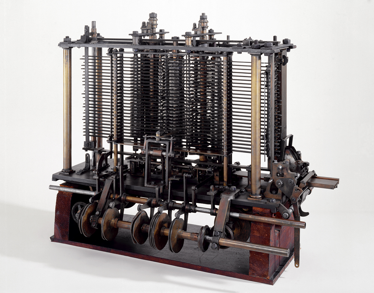
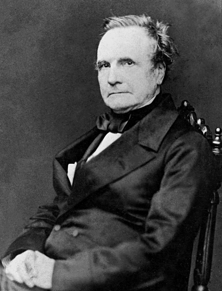
Charles Babbage’s Analytical engine (1837)
Turing complete. Programs on punch cards. Never fully built, a simplified version was built by his son later.

First program written by Ada Lovelace (computing Bernoulli numbers).

Calculating machine of Babbage’s Analytical Engine. Source: Wikimedia

Charles Babbage, 1860. Source: Wikimedia

Ada Lovelace, 1843. Source: Wikimedia

Percy Ludgate’s Analytical engine (1909)
Turing complete. Programs on punch cards.
Never built, designed independently from Babbage’s engine.

A Brief History of Computers and Operating Systems (2)

First generation: Electro-mechanical computers (1940 – 1955)

Heavy developments during World War II to help development of weapons (physical simulations) and compute rocket trajectories.

  • Zuse Z3 (1941, Germany): First Turing complete electro-mechanical computer (programs on punched 35 mm film)
  • Colossus Mark 1 (1943, UK): First programmable fully electronic computer (programmed with cables and switches)
  • ENIAC (1946, USA): First Turing complete fully electronic computer (programmed with cables and switches)
  • Manchester Baby (1948, UK): Turing complete, fully electronic, programs entered in memory via keyboard

Zuse Z3 (replica). Source: Wikimedia

Manchester Baby (replica). Source: Wikimedia

Theoretical work on computation theory and computer architectures, with Alan Turing and John von Neumann

First compiler by Grace Hopper (1952) for the UNIVAC I computer

Alan Turing, 1936.
Source: Wikimedia

John von Neumann, 1940s.
Source: Wikimedia

Grace Hopper, 1984.
Source: Wikimedia

No real operating systems, operators reserved the machines, programmed them or manually inserted the punch cards, and waited for the results.

A Brief History of Computers and Operating Systems (3)

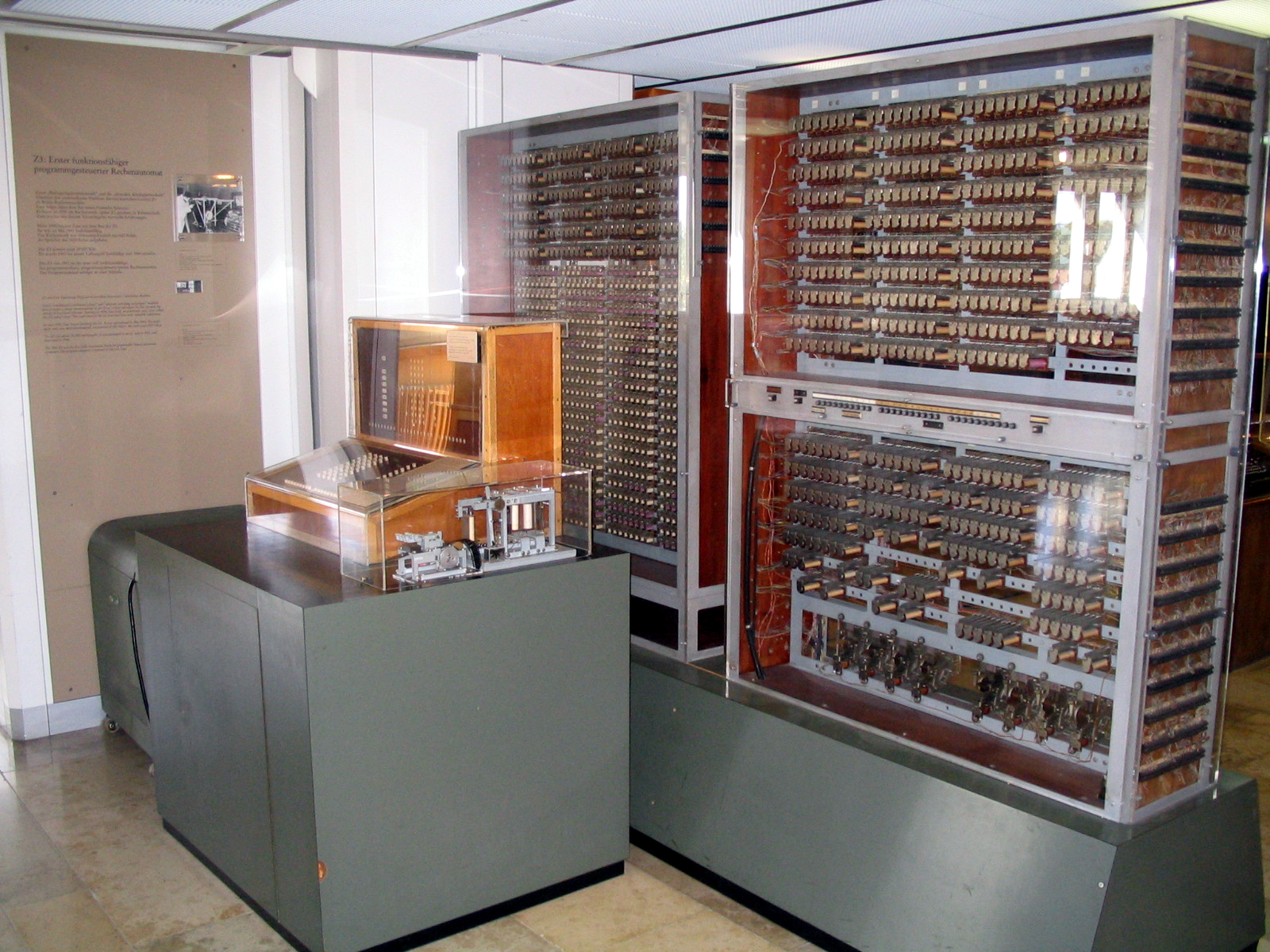
Second generation: Transistor computers (1955 – 1965)

With transistors, computer become reliable enough for commercial use
Mainframes are bought by corporations, government agencies and universities,
e.g., weather forecast, engineering simulation, accounting, etc.

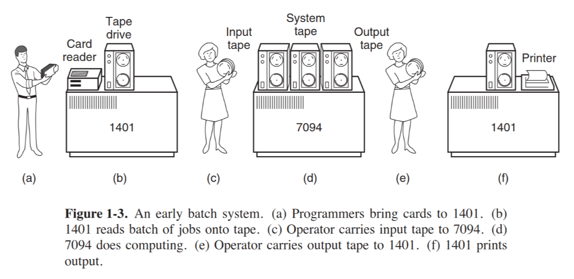
First real of operating systems with GM-NAA I/O (1956), IBSYS (1960), working in batch mode to schedule and pipeline jobs

Source: Modern Operating Systems, A. S. Tanenbaum, H. Bos, page 9.


Time sharing systems with CTSS (1961) and BBN Time-Sharing System (1962)

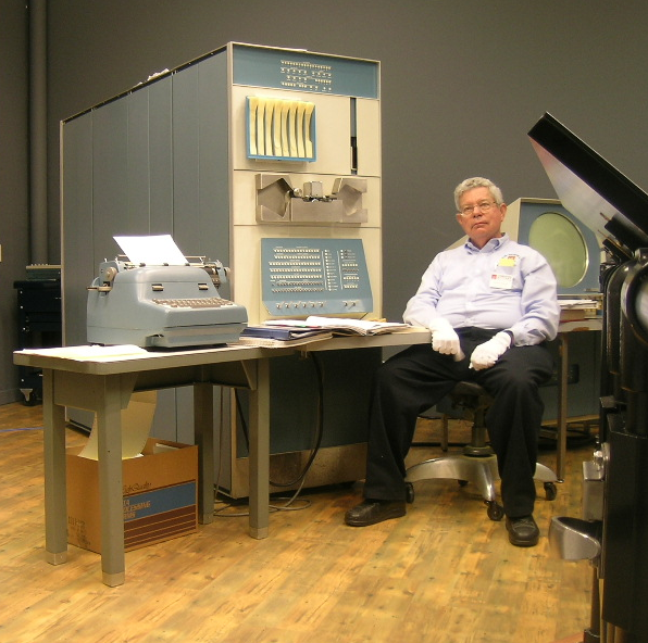
First minicomputers for individual users: PDP-1 (1961), LINC (1962)

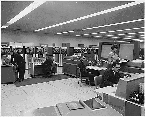
NASA computer room with two IBM 7090s, 1962. Source: Wikimedia

PDP-1 computer. Source: Wikimedia

A Brief History of Computers and Operating Systems (4)

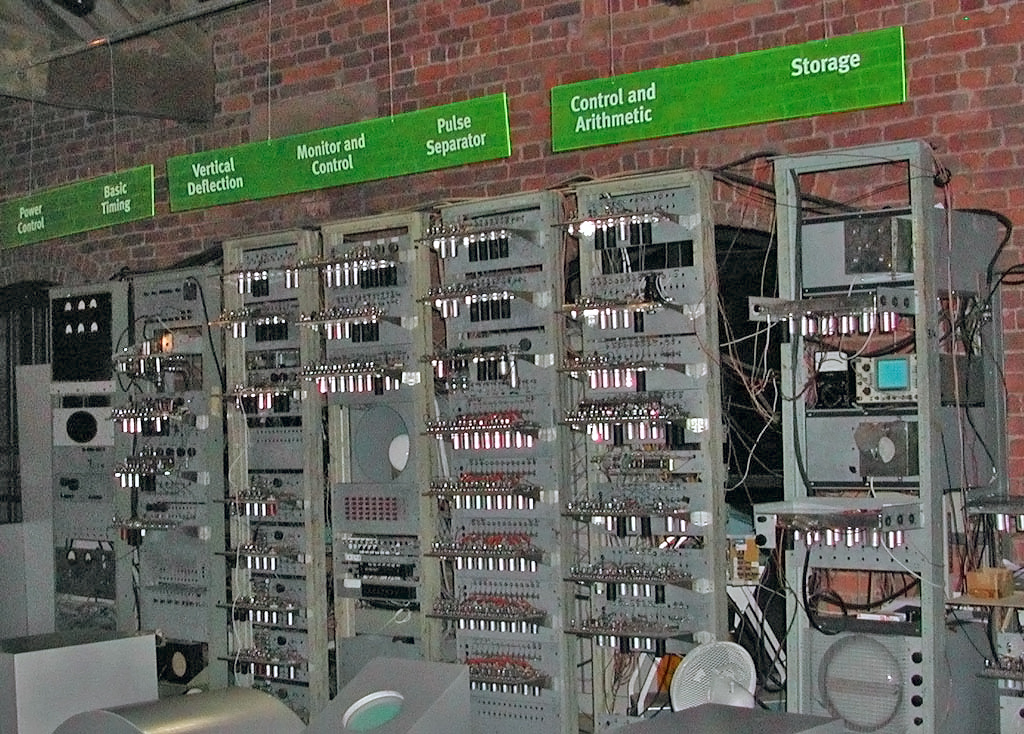
Third generation: Integrated circuits (1965 – 1980)

Minicomputers and mainframes are becoming more commonplace

IBM releases its OS/360 (1966) that features multiprogramming

MIT, Bell and General Electric develop Multics (1969) that pioneered a lot of common OS concepts
e.g., hierarchical file systems, protection domains, dynamic linking, processes

Bell (Ken Thompson, Dennis Ritchie, et al.) develop UNIX (1969-71) influenced by Multics, with novel concepts
e.g., “everything is a file” philosophy, inter-process communication (pipes), unified file systems

This later on led to the creation of the POSIX standard


UNIX will influence the design of many operating systems:

  • Berkeley’s BSD (1978)
  • AT&T’s System V (1983)
  • Vrije University’s MINIX (1987)
  • Linux (1991)

A Brief History of Computers and Operating Systems (5)

Third generation: Personal computers (1980 – today)

Large scale integration enabled to build chips with thousands of transistors/mm2 (hundreds of millions today)
Thus, microcomputers for personal use became powerful and affordable

1974: Intel releases the 8080, the first 8-bit general purpose CPU and the first disk-based OS: CP/M

1980: IBM designs the IBM PC and tasks Bill Gates (Microsoft) to find them a suitable OS
He purchases DOS (Disk Operating System) from a Seattle-based company and licenses it to IBM for the PC

1981: IBM releases the PC with MS-DOS as its operating system

1984: Apple releases the Macintosh with MacOS featuring a graphical user interface (GUI)
the first GUI was developed at Xerox, but they did not realize its potential, unlike Steve Jobs…

Fast forward to today:

  • Microsoft develops Windows
    • on top of MS-DOS: Windows 1.0 to 3.1, Windows 95, 98, ME
    • with the Windows NT family: NT, 2000, XP, Vista, 7, 8, 10, 11
  • Apple continues to develop macOS:
    • Mac OS versions 1 to 9 (2001)
    • Mac OS X (and now macOS) with a new hybrid kernel (2001 – today)
    • iOS, iPadOS, watchOS
  • Linux is everywhere on the server market and embedded devices, e.g., Android

A Quick Review of Computing Hardware

Overview

A computer system is a set of chips, devices and communication hardware.


It comprises:

  • Computing hardware that executes programs
    Central Processing Unit (CPU)
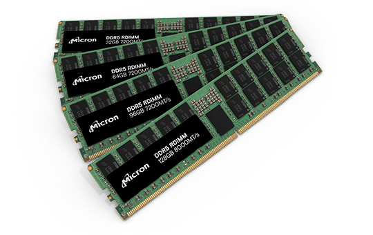
  • Memory to store volatile information with fast access
    Random Access Memory (RAM), caches
  • Various device controllers to communicate with hardware devices using different specifications
    Disk, video, USB, network, etc.
  • A communication layer that enables all these components to communicate commands and data
    Bus


Central Processing Unit

The Central Processing Unit, or CPU/processor, is the brain of the computer.
Its job is to load an instruction from memory, decode and execute it, and then move on to the next instruction and repeat.
Each CPU understands one “language”, its instruction set, e.g., x86, ARMv7, which makes them not interoperable.

A CPU contains the following components:

  • Execution units that execute instructions
    • Decoder reads an instruction and forwards to the proper execution unit
    • Arithmetic/Logical Unit (ALU) performs integer and binary operations
    • Floating-Point Unit (FPU) performs floating-point operations
    • Memory Unit (MU) performs memory accesses
  • Registers that store data
    • State information, e.g., instruction pointer, stack pointer, return address
    • Program values in general-purpose registers
  • Multiple levels of caches to avoid performing redundant and costly memory accesses

Memory and Devices

The CPU is the “brain” of the computer and acts “by itself” (following the running program instructions).
The other components act as they are instructed by the CPU.

  • Memory is a passive device that stores data. The CPU and devices read from and write to it.
  • Other devices perform operations as instructed by the CPU.
    e.g., display something on the monitor, send this through the network, etc.

Communication between components happens through the bus, the communication layer that links them.


Protection Domains and Processor Privilege Levels

The Need for Isolation

Some operations are critical and could break the system if done improperly:

  • Modify the state of a device
    e.g., modify the state of the microphone LED to make it look muted when it is not
    e.g., make a USB drive read-only/writable
  • Access restricted memory areas
    e.g., modify a variable from another program
    e.g., read private data – passwords – from other programs

We cannot trust all application software to not do these critical operations!


User applications can be written by anyone:

  • Programmers lacking skills/experience/knowledge
  • Malicious programmers that want to attack a system

The operating system needs to isolate these operations to make the system safe and secure!

Protection Domains

In order to provide the necessary isolation, operating systems provide different protection domains or modes.

These domains give different capabilities to the code executing on the machine.


Usually, two protection domains are provided:

  • Supervisor mode
  • User mode

They have different privilege levels, allowing or restricting a set of operations.


Info

Protection domains are software-defined by the operating system.

The OS relies on hardware features to be enforce them. (We will discuss these features later on.)

Supervisor Domain

Supervisor domain (also referred to as S mode) has the highest privilege level.

This means that all operations are allowed.


Programs running in this domain can:

  • Use all the instruction set defined by the CPU architecture
  • Directly interact with hardware devices
  • Access any memory area


This domain is used by the kernel that contains the low level components of the operating system.

User Domain

User domain (also referred to as U mode) has the lowest privilege level.

This means that some operations are restricted in this domain.


Programs running in this domain cannot:

  • Use privileged instructions that modify the system state,
    e.g., directly manipulate a hardware device
  • Access some memory areas,
    e.g., access the memory of another program


This domain is used by all the applications outside of the kernel:
high level operating system services and user applications.

Relationship Between Protection Domains

User mode is usually a subset of supervisor mode.

All the operations that can be performed in user mode can also be performed in supervisor mode.


Protection domains are usually enforced with features provided by the hardware.

Processor Privilege Levels

In practice, protection domains are backed by hardware processor privilege levels, also called CPU modes or CPU states.

For example, x86 provides four levels, also called protection rings.

ARMv7 provides three privilege levels, while ARMv8 provides four.


x86 protection rings

ARMv7 privilege levels

Careful with the numbers!

There is no standard order in the value of the levels! For x86, ring 0 is the most privilege, while PL0 is the least privileged on ARMv7!

Matching Protection Domains to Privilege Levels

Most operating systems use two protection domains (user and supervisor), e.g., Linux, Windows, macOS.
Thus, they only need two processor privilege levels, as specified by the Instruction Set Architecture:


Protection domains and protection rings on x86 platforms

Protection domains and privilege levels on ARMv7 platforms


Virtualized context

In virtualized environments, the hypervisor needs specific instructions.
On x86, they are in a new ring -1 level, while ARMv7 uses its PL2 level.

Switching Between Modes

When applications running in user mode need to use a privileged feature, they have to switch to supervisor mode.

        e.g., writing to a file on disk, allocating memory, etc.


This switching is performed through system calls, which are function calls from user to supervisor mode.
They provide a controlled interface between user space applications and privileged operating system services.
This ensures that user applications can perform privileged operations in a secure way, only through kernel code.

Examples: read() and write() for file manipulation, listen(), send() and receive() for networking


In addition to calling the function, a system call also checks that:

  • The program is allowed to perform this request
    e.g., the program is not trying to manipulate a resource it is not allowed to access
  • The arguments passed by the program are valid
    e.g., the program is not trying to get privileged information with a forged pointer

Important

During a system call, the user program switches to supervisor mode to execute privileged code!

The user program does not “ask the kernel” to do something!

Protection Domains and Operating System Architecture

Let’s go back to our operating system architecture and add the protection domains.

User applications and high level operating system services run in user mode.

The kernel runs in supervisor mode.


What components of the operating system are in the kernel?

Operating System Architectures

Supervisor or User Mode? That Is the Question

When designing an operating system, one main question has to be answered:

Which component will run in supervisor mode (and which in user mode)?

In other words:

Which components of the operating system are part of the kernel?


Some components have to be in the kernel because they need privileged instructions.
Other components can reside anywhere. Their position will have an impact on safety, performance and API.


There are four main architectures:

  • Monolithic kernels
  • Microkernels
  • Hybrid kernels
  • Unikernels

Let’s have a look at these different architectures!

Monolithic Kernels

A monolithic kernel provides, in kernel space, a large amount of core features, e.g., process and memory management, synchronization, file systems, etc., as well as device drivers.


Characteristics

  • Defines a high level interface through system calls
  • Good performance when kernel components communicate (regular function calls in kernel space)
  • Limited safety: if one kernel component crashes, the whole system crashes

Examples

  • Unix family: BSD, Solaris
  • Unix-like: Linux
  • DOS: MS-DOS
  • Critical embedded systems: Cisco IOS

Modularity

Monolithic kernels can be modular and allow dynamic loading of code, e.g., drivers. These are sometimes called modular monolithic kernels.

Source: Wikimedia

Microkernels

A microkernel contains only the minimal set of features needed in kernel space: address-space management, basic scheduling and basic inter-process communication.
All other services are pushed in user space as servers: file systems, device drivers, high level interfaces, etc.


Characteristics

  • Small memory footprint, making it a good choice for embedded systems
  • Enhanced safety: when a user space server crashes, it does not crash the whole system
  • Adaptability: servers can be replaced/updated easily, without rebooting
  • Limited performance: IPCs are costly and numerous in such an architecture

Examples

  • Minix
  • L4 family: seL4, OKL4, sepOS
  • Mach
  • Zircon

Source: Wikimedia

Hybrid Kernels

The hybrid kernel architecture sits between monolithic kernels and microkernels.
It is a monolithic kernel where some components have been moved out of kernel space as servers running in user space.

While the structure is similar microkernels, i.e., using user servers, hybrid kernels do not provide the same safety guarantees as most components still run in the kernel.

Controversial architecture

This architecture’s existence is controversial, as some just define it as a stripped down monolithic kernel.


Examples

  • Windows NT
  • XNU (Mach + BSD)

Source: Wikimedia

Unikernels

A unikernel, or library operating system, embeds all the software in supervisor mode.
The kernel as well as all user applications run in the same privileged mode.

It is used to build single application operating systems, embedding only the necessary set of applications in a minimal image.


Characteristics

  • High peformance: system calls become regular function calls and no copies between user and kernel spaces
  • Security: attack surface is minimized, easier to harden
  • Usability: hard to build unikernels due to lack of features supported


Examples

  • Unikraft
  • clickOS
  • IncludeOS

Comparison Between Kernel Architectures


The choice of architecture has various impacts on performance, safety and interfaces:

  • Switching modes is costly: minimizing mode switches improves performance
  • Supervisor mode is not safe: minimizing code in supervisor mode improves safety and reliability
  • High level interfaces for programmers are in different locations depending on the architecture
    i.e., in the kernel for monolithic, but in libraries or servers for microkernels

Recap

Recap

  1. Definition
    The operating system is the software layer that lies between applications and hardware.
    It provides applications simple abstractions to interact with hardware and manages resources.
    It usually offers the following services: program management, memory management, storage management, networking and human interface.

  2. Protection domains
    Supervisor mode for critical operations in the kernel, user mode for the non-critical OS services and user applications.
    Hardware enforces these with processor privilege levels.
    System calls allow user mode applications to use supervisor mode services.

  3. Kernel architectures
    Monolithic, microkernel, hybrid, unikernel.


Next week, we will start diving into program management in the OS with processes and threads!

Chapter 2: Program Execution

This Week’s Program

We will explore how programs are managed and executed by the operating system:

  1. Processes
    Abstraction of a program, process control block, states
  2. Threads
    Abstraction of a unit of execution, user vs. kernel threads, multi-threading
  3. Scheduling
    General concepts, batch, interactive, real time

Processes

One System, Multiple Programs

Your system runs a large number of applications at the same time:

  • E-mail client
  • Web browser(s)
  • Music player
  • Development environment


In such a multiprogramming system, there will be more programs than CPUs available to run them.

The job of the OS is to switch between programs very quickly, every tens or hundreds milliseconds, to give the illusion of parallelism.


The OS needs to keep track of each running program to manage them properly!

The Process Model

Definition

A process is the abstraction that represents an instance of a running program.

Processes contain the set of information required for the program to execute properly:

  • Code (the binary representation of the program’s instructions)
  • Memory (variables, stack, heap, etc.)
  • Registers (instruction pointer, stack pointer, etc.)
  • Resources in use (open files, sockets, etc.)

They are independent entities that the OS manipulates, choosing which one to run and when.

Caution

Program \(\neq\) process! The program is the ‘recipe’ (the code) and the process is an execution of the program.

Process Creation

A new process can be created for various reasons:

  • A user creates it by starting a new program
    e.g., by clicking on the icon or starting it from the command line
  • Another process creates it using a process creation system call
    e.g., your web browser starts your PDF reader after downloading a file
  • When the system starts
    an initial process is created to initialize the system, launch other programs like the desktop environment, etc.


Depending on their purpose, processes can be classified as:

  • Foreground processes that interact with the user
    e.g., video player, calculator, etc.
  • Background processes that run by themselves with no user interaction required
    e.g., weather service, notification service, network configuration, etc.

Note

Background processes that always stay in the background are also called daemons or services.

Process Hierarchy

Most systems keep an association between a process and the process that created it, its parent.


In UNIX-based systems, all processes are linked in this way, creating a process tree.
The root of the tree is init, the first process created when the system boots.

init init thermald thermald init--thermald bluetoothd bluetoothd init--bluetoothd sshd sshd init--sshd cupsd cupsd init--cupsd gnome GNOME init--gnome netman NetworkManager gnome--netman thunderbird thunderbird gnome--thunderbird firefox firefox gnome--firefox vscode vscode gnome--vscode term gnome-terminal gnome--term firefox1 firefox-tab1 firefox--firefox1 firefox2 firefox-tab2 firefox--firefox2 firefox3 firefox-tab3 firefox--firefox3 vscode1 vscode-win1 vscode--vscode1 vscode2 vscode-win2 vscode--vscode2 ssh ssh term--ssh emacs emacs term--emacs


The init process also adopts orphaned processes.
e.g., if gnome-terminal terminates without terminating its child processes (ssh and emacs),
they become children of init


Windows does not keep a full process tree.
Parent processes are given a handle on their children.
The handle can be passed on to another process.

Process States

After its creation, a process can go into three different states:

  • Ready (also called runnable)
    The process can be executed and is waiting for the scheduler to allocate a CPU for it
  • Running
    The process is currently being executed on the CPU
  • Blocked
    The process cannot run because it is waiting for an event to complete


State transitions:

  1. Process creation ( \(\emptyset \rightarrow\) ready)
  2. Scheduler picks the process to run on the CPU (ready \(\rightarrow\) running)
  3. Scheduler picks another process to run on the CPU (running \(\rightarrow\) ready)
  4. Process cannot continue to run, waiting for an event (running \(\rightarrow\) blocked)
    e.g., keyboard input, network packet, etc.
  5. Blocking event is complete, the process is ready to run again (blocked \(\rightarrow\) ready)

Process Execution Patterns and Scheduling

Processes have different behaviors depending on the program they execute.


  • A command line interpreter (CLI) repeatedly:
    • Waits for a user to type in commands (running \(\rightarrow\) blocked)
    • Wakes up and executes them when available (blocked \(\rightarrow\) ready \(\leftrightarrow\) running)
  • A video player repeatedly:
    • Reads data from disk and waits for it to be available in memory (running \(\rightarrow\) blocked)
    • Copies the frames into graphical memory (blocked \(\rightarrow\) ready \(\leftrightarrow\) running)
  • A program that computes digits of \(\pi\) never waits and only uses the CPU (ready \(\leftrightarrow\) running)

Definition

The scheduler is the component of the OS that manages the allocation of CPU resources to processes, depending on their state.

Process Implementation

For each process, the OS maintains a process control block (PCB) to describe it.


Process Memory Layout

A process’ memory, or address space, is split into several sections.

  • Kernel memory is shared between all processes, accessible only in supervisor mode
    In 32 bit Linux, 1 GB for the kernel, 3 GB for user space.
    In 64 bit Linux, 128 TB for the kernel, 128 TB for user space
  • Text is where the program binary is loaded in memory
    It contains the actual binary instructions that will be executed by the CPU.
  • Data contains the static initialized variables from the binary
    Initialized global variables and static local variables, constant strings
    e.g., a global \(~~~~\) int count = 0; \(~~~~\) or a local \(~~~~\) static int idx = 0;
  • BSS (block starting symbol) contains static uninitialized variables
    e.g., a global \(~~~~\) static int i;
  • Heap contains dynamically allocated memory, grows towards higher addresses
    e.g., malloc(), brk/sbrk, mmap()
  • Stack contains local variables, environment variable, calling context (stack frame)
    Grows towards address 0x00000000

Process Registers

Registers are the part of the process state that are physically on the CPU

  • Instruction Pointer (IP), or Program Counter (PC)
    Contains the address of the next instruction to execute if not jumping
    x86-64: RIP
    arm64: PC
  • Stack Pointer (SP)
    Contains the address of the top of the stack
    x86-64: RSP
    arm64: SP
  • General Purpose (GP)
    Contains values or addresses used by instructions
    x86-64: RAX, RBX, …, R15
    arm64: X0–X30
  • Page Table Pointer
    Contains the address of the memory mapping
    x86-64: CR3
    arm64: TTBR

We’ll come back to how memory mappings and page tables work in a future lecture.

Context Switch

When the OS changes the currently running process, it performs a context switch.

The OS needs to exchange the PCB of the current process with the PCB of the next process.


Context switching between the running process A and the ready process B happens in several steps:

  1. Change the state of the currently running process A to ready
  1. Save the CPU registers into A’s PCB
  1. Copy the registers from B’s PCB into the CPU registers
  1. Change the state of B from ready to running


Process Isolation

Another property of processes is that they are isolated from each other.
They act independently, as if they were running alone on the machine.

They do not share memory, open files, etc.


We will see how this is enforced later when discussing memory and file management.


Multiprocessing

Processes can communicate and collaborate if explicitly stated in the program.
We will discuss that in a future lecture.

POSIX API: Processes

Let’s quickly see the POSIX API to manage processes in C.


pid_t fork(void);
Create a new process by duplicating the calling process, i.e., its PCB and memory.
Upon success, returns the PID of the child in the parent, 0 in the child. Returns -1 upon error.


int exec[lvpe](const char *path, const char *arg, ...);
This family of functions replaces the current program with the one passed as a parameter.
Returns -1 upon error. Upon success, it doesn’t return, but the new program starts.


pid_t wait(int *status);
Wait for any child process to terminate or have a change of state due to a signal.
Returns the PID of the child on success, -1 on failure.

POSIX API: Processes – Example

fork.c
#include <stdio.h>
#include <stdlib.h>
#include <unistd.h>
#include <sys/wait.h>

int main(int argc, char **argv)
{
    pid_t pid;

    printf("Parent PID: %d\n", getpid());

    pid = fork();
    switch (pid) {
    case -1:
        printf("[%d] Fork failed...\n", getpid());
        return EXIT_FAILURE;
    case 0:
        printf("[%d] I am the child!\n", getpid());
        sleep(3);
        printf("[%d] I waited 3 seconds\n", getpid());
        break;
    default:
        printf("[%d] Fork success, my child is PID %d\n", getpid(), pid);
        wait(NULL);
        printf("[%d] Child has terminated, wait is over\n", getpid());
    }

    return EXIT_SUCCESS;
}
❱ gcc -o fork fork.c
❱ ./fork                
Parent PID: 254
[254] Fork success, my child has PID 255
[255] I am the child!
[255] I waited 3 seconds
[254] Child has terminated, wait over

Processes: A Heavyweight Mechanism

Applications may benefit from executing multiple tasks at the same time,
e.g., your development environment needs to wait for keyboard input, perform syntax check, render the UI, run extensions, etc.


Using one process per task is not always a good idea!


Creating a process means copying an existing one

\(\rightarrow\)

It is a costly operation!

Processes don’t share memory

\(\rightarrow\)

\(\rightarrow\)

Good for isolation.

Communication must be explicitly set up!


Is there a more lightweight mechanism to execute parallel programs?

Threads

Definition

A thread is the entity that executes instructions. It has a program counter, registers and a stack.

A process contains one or more threads, and threads in the same process share their memory.

Threads are sometimes called lightweight processes.


Info

Another definition of a process is a set of threads sharing an address space.
But we will discuss that definition in future lectures when explaining memory management and virtual memory.

Process Model and Thread Model

Let’s go back to our process model, and add threads in the mix.

Processes group resources together, e.g., memory, open files, signals, etc., while threads execute code.


Example 1: Multithreaded web server

The main thread creates worker threads to handle requests.

Example 2: Multithreaded text editor

The program creates a thread for each task that has to run in parallel.

Threads: Shared vs. Private Data

Threads in the same process share some resources, while others are thread-private.


Per-process resources

Address space
Global variables
Open files
Child processes
Pending alarms
Signals and signal handlers
Accounting metadata

Per-thread resources

Program counter
Registers
Stack
State

Threading Implementation

Threads are usually implemented as a thread table in the process control block.


POSIX API: Threads

Let’s have a quick look at the main functions of the POSIX API to manipulate threads:


int pthread_create(pthread_t *thread, const pthread_attr_t *attr, void *(*function)(void *), void *arg);
Create a new thread that will execute function(arg).


void pthread_exit(void *retval);
Terminate the calling thread.


int pthread_join(pthread_t thread, void **retval)
Wait for thread to terminate.


Note

You need to link the pthread library when compiling your programs, by passing the -pthread option to your compiler.

POSIX API: Threads – Example

pthread.c
#define _GNU_SOURCE
#include <stdio.h>
#include <stdlib.h>
#include <unistd.h>
#include <pthread.h>

void *fn(void *arg)
{
    printf("[%d] String: %s, sleeping 3s now...\n", gettid(), arg);
    sleep(3);
    return NULL;
}

int main(int argc, char **argv)
{
    pthread_t worker;
    int ret;

    printf("[%d] Creating worker...\n", gettid());
    
    ret = pthread_create(&worker, NULL, fn, argv[0]);
    if (ret != 0) {
        perror("pthread_create failed\n");
        return EXIT_FAILURE;
    }

    printf("[%d] Waiting for worker thread...\n", gettid());
    pthread_join(worker, NULL);
    printf("[%d] Joined worker thread\n", gettid());

    return EXIT_SUCCESS;
}
❱ gcc -o pthread pthread.c -pthread
❱ ./pthread          
[333] Creating worker...
[333] Waiting for worker thread...
[334] String: ./pthread, sleeping 3s now...
[333] Joined worker thread  

User-Level Threads

Threading can also be handled at the user level:

  • This allows programs to use the thread model on OSes that do not support threads
  • Scheduling can be performed by the program instead of the OS


It is usually provided by:

  • Programming languages, e.g., Go, Haskell, Java
  • Libraries, e.g., OpenMP, Cilk, greenlet


These runtime systems (programming language or library) must perform a form of context switching and scheduling.

Thread Mapping Models

The OS only manipulates its own threads, i.e., kernel threads, it has no notion of user-level threads.

Thus, user-level threads must be attached to these underlying kernel threads: this is called the thread mapping model.


There are three thread mapping models mapping user to kernel threads:

  • 1:1
  • N:1
  • N:M

Thread Mapping Models – 1:1

Each user thread is mapped to a single kernel thread.

Every time a user thread is created by the application, a system call is performed to create a kernel thread.

Threading is completely handled by the OS, thus requiring OS support for threading.


Pros/Cons:

+ Parallelism

+ Ease of use

- No control over scheduling


Examples: Pthread C library, most Java VMs

Thread Mapping Models – N:1

All user threads are mapped to a single kernel thread.

Every time a user thread is created, the user runtime maps it to the same kernel thread.

The OS doesn’t know about user threads, and doesn’t need to support threads at all.

The runtime system must manage the context switches, scheduling, etc.


Pros/Cons:

+ Full scheduling control

~ Reduced context switch overhead

- No parallelism


Examples: Coroutines in Python, Lua, PHP

Thread Mapping Models – N:M

Multiple user threads (\(N\)) are mapped to multiple kernel threads (\(M\)).

Flexible approach that provides the benefits of both 1:1 and N:1 models, at the cost of complexity.

The runtime system manages the scheduling and context switches of user threads,
while the OS (kernel) manages the scheduling and context switches of kernel threads.


Pros/Cons:

+ Parallelism

+ Control over the scheduling

- May be complex to manage for the runtime

- Performance issues when user and kernel schedulers make conflicting decisions


Examples: goroutines in Go, Erlang, Haskell

Usual implementation

The runtime system statically creates one kernel thread per core, and schedules an arbitrary number of user threads on them.

User Threads and Blocking Operations

When multiple user threads share a kernel thread, they share the kernel threads’s state.

If a user thread performs a blocking operation, e.g., reading from the disk, all shared user threads are also blocked.


Two main ways of avoiding this issue:

  • Replace all blocking operations with asynchronous operations and wait-free algorithms.
    This can be done explicitly by programmers, thus increasing the code complexity, or transparently by the runtime system or the compiler.
  • Rely on cooperative multithreading, similar to coroutines in language theory.
    This type of user threads is also called fibers.

Scheduling

The Scheduler

Definition

The scheduler is the operating system component that allocates CPU resources to threads.
It decides which thread runs on which CPU, when and for how long.


The scheduling algorithm (or policy) used to take these decisions depends on:

  • The system itself, i.e., how many CPUs, how much memory, etc.
  • The workloads running on it, i.e., interactive applications, long running programs, etc.
  • The goals to achieve, i.e., responsiveness, energy, performance, etc.

Application Behavior

Each application has its own behavior depending on what it does.
But most of them alternate computations (on the CPU, ready or running) and waiting on IOs (blocked), e.g., waiting for data from disk.


There are two main classes of applications:

  • CPU-bound (or compute-bound): long computations with a few IO waits
    e.g., data processing applications
  • IO-bound: short computations and frequent IO waits
    e.g., web server forwarding requests to worker threads

Triggering the Scheduler

Depending on the applications’ and the hardware’s behaviors, the scheduler decides which thread runs on which CPU.


Application behavior:

  1. When a process/thread is created ( \(\emptyset \rightarrow\) ready), i.e., after a fork()/pthread_create()
    \(\implies\) Does the parent or child thread run first?
  2. When a thread terminates (ready/running \(\rightarrow\) X)
    \(\implies\) Which thread runs next?
  3. When a thread waits on for an IO to complete (running \(\rightarrow\) blocked), e.g., waiting on a keyboard input
    \(\implies\) Which thread runs next?


Hardware behavior:

  1. An IO completes, triggering an interrupt and waking a thread (blocked \(\rightarrow\) ready), e.g., data request from the disk is ready, network packet arrival, etc.
    \(\implies\) Let the current thread run or replace it with the waking thread?
  2. A clock interrupt occurs
    \(\implies\) Preemption?

Preemption

An important characteristic of a scheduler is whether it is preemptive or not.


Definition

A preemptive scheduler can forcefully interrupt a running task to execute a different one.


In other words:

  • Non-preemptive schedulers choose a thread to run and let it run until it blocks, terminates or voluntarily yields the CPU
  • Preemptive schedulers might stop a running thread to execute another one after a given period of time or a given event


Note

Preemption is only possible on systems with support for interrupts (we will see that in a future chapter).

Categories of Scheduling Algorithms

Depending on the system, workloads and goals of the system, different categories of algorithms should be used:


  • Batch: Business applications, with long running background tasks (compute-bound)
    e.g., accounting, file conversion/encoding, training machine learning models, etc.
    \(~~~~~\longrightarrow\) Usually no preemption to minimize scheduling overhead


  • Interactive: Users are interacting with the system, or IO-bound applications
    e.g., text editor, web server, etc.
    \(~~~~~\longrightarrow\) Preemption is necessary for responsiveness


  • Real time: Constrained environments, where deadlines must be met
    e.g., embedded systems
    \(~~~~~\longrightarrow\) May or may not have preemption, as these systems are usually fully controlled, with no arbitrary programs running

Scheduling Metrics

Depending on the workloads, different goals are desirable for the scheduling algorithm.
In other words, the scheduler can optimize different metrics depending on requirements.


All categories

  • Fairness: Processes should get a similar amount of CPU resource allocated to them. Fairness is not equality, the amount of CPU allocation can be weighted, e.g, depending on priority
  • Resource utilization: Hardware resources, e.g., CPU, devices, should be kept busy as much as possible

Interactive

  • Response time/latency: Respond to requests quickly
  • User experience: The system should feel responsive to users


Batch

  • Throughput: Maximize the number of jobs completed per unit of time, e.g., packets per second, MB/s, etc.
  • Turnaround time: Minimize the duration between job submission and completion
  • CPU utilization: Keep the CPU busy as much as possible

Real time

  • Meeting deadlines: Finish jobs before the requested deadlines to avoid safety problems
  • Predictability: Behave in a deterministic manner, easy to model and understand

Example of Scheduling Policies

Now, let’s have a look at some scheduling policies!


Batch

  • First-Come First-Served (FCFS)
  • Shortest Job First (SJF)
  • Shortest Remaining Time (SRT)

Interactive

  • Round-Robin (RR)
  • Priority-based
  • Fair
  • Lottery

Real time

For each policy, we will give the following characteristics:

  • Runqueue: How are the ready threads stored/organized?
  • Election: What happens when the scheduler must choose a new thread to execute?
  • Block: What happens when a running thread becomes blocked?
  • Wake up: What happens when a thread wakes up from being in a blocked state to become ready?

Batch Scheduling: First-Come, First-Served

The First-Come, First-Served (FCFS) scheduler assigns threads to CPUs in their order of arrival, in a non-preemptive way.


Runqueue: Threads are stored in a list sorted by order of arrival, with the first element being the oldest

Election: Choose the head of the runqueue

Block: Remove the thread from the runqueue and trigger an election

Wake up: Add the thread to the runqueue (at the end, like a newly created thread)


Event

Initial state

Election

\(A\) waits on an IO

\(A\) wakes up

\(B\) terminates

\(E\) starts

Running

\(\emptyset\)

\(A\)

\(B\)

\(B\)

\(C\)

\(C\)

Runqueue

\(A \rightarrow B \rightarrow C \rightarrow D\)

\(B \rightarrow C \rightarrow D\)

\(C \rightarrow D\)

\(C \rightarrow D \rightarrow A\)

\(D \rightarrow A\)

\(D \rightarrow A \rightarrow E\)


Pros

Easy to implement

Cons

With many threads, long latencies for IO-bound threads and high turnaround time for CPU-bound threads

Batch Scheduling: Shortest Job First

The Shortest Job First (SJF) scheduler assumes that a job’s run time is known in advance.
It works in the same way as FCFS, except that the job queue is sorted by run time.


Runqueue: Threads are stored in a list sorted by increasing total duration

Election: Choose the head of the runqueue

Block: Remove the thread from the runqueue and trigger an election

Wake up: Add the thread to the runqueue (at its sorted position)


Example:

Let’s assume four tasks \(A, B, C\) and \(D\), arriving in that order and the following known durations: \(A = 5\), \(B = 3\), \(C = 4\), \(D = 3\)

Note

Total turnaround time \(= a + b + c + d\)

Average turnaround time \(= \frac{4a + 3b + 2c + d}{4}\)

Policy Total turnaround Average turnaround
FCFS 15 10
SJF 15 8.5

Pros

Optimal when all jobs are known in advance

Cons

Does not adapt well to deffered job arrivals

Batch Scheduling: Shortest Remaining Time

The Shortest Remaining Time (SRT) scheduler is a modified preemptive version of SJF, where jobs are sorted by their remaining run time.


Runqueue: Threads are stored in a list sorted by increasing remaining duration

Election: Choose the head of the runqueue

Block: Remove the thread from the runqueue and trigger an election

Wake up: Add the thread to the runqueue (at its sorted position). If it has a lowest remaining time than the running thread, preempt it

Pros

Short deferred jobs are not penalised

Cons

Long jobs can be delayed infinitely by new short jobs

Interactive Scheduling: Round-Robin

Round robin is a simple preemptive scheduler.
Each thread is assigned a time interval (quantum) during which it is allowed to run.
When a thread uses up its quantum, it is preempted and put back to the end of the queue.


Runqueue: Threads are stored in a list

Election: Choose the head of the runqueue. Election is also triggered when the running thread uses up its quantum

Block: Remove the thread from the runqueue and trigger an election

Wake up: Add the thread to the runqueue (optionally refilling its quantum)


Example: quantum = 4ms; four tasks \(A, B, C\) and \(D\)


\(A\) is chosen as the head of the list to become running, with a quantum of 4 ms
\(B\) becomes the new head, i.e., the next thread to run after \(A\)

\(A\) runs for 4 ms (using up its quantum), then gets preempted
\(B\) is the new running thread
\(A\) becomes ready and is put at the end of the queue

\(B\) runs for 2 ms, then waits on an IO (becoming blocked)
\(C\) becomes running in its place
\(B\) is not put back in the queue as it is not ready
\(D\) will be the next scheduled thread

The IO \(B\) was waiting for is done, so \(B\) becomes ready again
\(B\) is inserted at the end of the queue
\(C\) keeps running until the end of its quantum

\(C\) finishes its 4 ms quantum and gets preempted
\(D\) is the new running thread
\(C\) is put back at the end of the queue as ready

Pros

Easy to implement, relatively fair

Cons

Quantum must be chosen carefully, requiring fine tuning

Note

The first versions of Linux used this algorithm.

Interactive Scheduling: Priority-based

Each process is assigned a priority, and the priority-based scheduler always runs the thread with the highest priority.
Priorities might be decided by users or by the system depending on the thread behavior (IO- or compute-bound).


Runqueue: Threads are stored in a list sorted by priority

Election: Choose the head of the runqueue (thread with the highest priority)

Block: Remove the thread from the runqueue and trigger an election

Wake up: Add the thread to the runqueue (at its priority)


Example: Multilevel queueing (or MLQ).

Multilevel feedback queueing

The system may change priorities to avoid threads hogging the CPU or starvation, and assign a quantum to threads to improve fairness.

Pros

High priority threads are not hindered by others

Cons

Not very fair, may be complex to tune the priorities

Note

Linux used a variation for years, and Windows still does.

Interactive Scheduling: Fair

A fair scheduler tries to give the same amount of CPU time to all threads.
Some may also enforce fairness between users (so-called fair-share schedulers),
e.g., user A starts 9 threads, user B starts 1 thread, they should still get 50% of the CPU each.


Runqueue: Threads are stored in a list sorted by used run time (how they have used the CPU)

Election: Choose the head of the runqueue (thread that used the least amount of CPU time)

Block: Remove the thread from the runqueue and trigger an election

Wake up: Add the thread to the runqueue (at its sorted position)


Usually, these schedulers also weight the fairness, e.g., with priorities.


Example: The Linux scheduler (CFS, now EEVDF)

Pros

Fairness

Cons

Usually complex implementation, with a lot of heuristics

Interactive Scheduling: Lottery

A lottery scheduler randomly chooses the next thread running on the CPU.
The randomness can be skewed by giving more lottery tickets to higher priority threads.


Runqueue: Threads are stored in a list, not sorted

Election: Randomly choose a thread from the runqueue

Block: Remove the thread from the runqueue and trigger an election

Wake up: Add the thread to the runqueue


Pros

Very simple implementation, randomness is pretty fair

Cons

Low control over the results of the scheduling

Real Time Scheduling

Real time schedulers must enforce that threads meet their deadlines.
They can be separated in two classes:

  • Hard real time: Deadlines must be met or the system breaks
    e.g., the brake system of a car must respond to the pedal being pressed very quickly to avoid accidents.
  • Soft real time: Deadlines can be missed from time to time without breaking the system
    e.g., a video player must decode 50 frames per second, but missing a frame from time to time is fine.


Real time applications may also be:

  • Periodic: the task periodically runs for some (usually short) amount of time,
    e.g., the frame decoder of the video player is started every 20 ms and must complete in less than 5 ms.
  • Aperiodic: the task occurs in an unpredictable way,
    e.g., the brake mechanism of a car is triggered when the pedal is pressed and must engage the brakes in less than 1 ms.


Examples of real time schedulers: Earliest Deadline First (EDF), Deadline Monotonic, etc.

Recap

Recap

  1. Processes
    Abstraction that represents a program in execution.
    It contains all the resources needed to run a program: memory, files, and threads.
    Processes are isolated from each other, and do not share resources, unless explicitly done.
  2. Threads
    Entity that executes code within a process.
    Threads share the resources of the process they belong to, but have their own state: program counter, registers and stack.
  3. Scheduling
    The scheduler is the OS component that allocates CPU resources to threads.
    It decides which thread runs on which CPU, when and for how long.
    Scheduling algorithms can be preemptive or not, and can be optimized for different workloads and goals.
  4. Scheduling policies
    Different scheduling policies exist, depending on the workloads and goals of the system.
    They can be batch, interactive or real time.
    Batch policies are usually non-preemptive, while interactive policies are preemptive.
    Real time policies can be preemptive or not, depending on the system.

Chapter 3: Memory Management

Overview

  1. Why is memory management needed?
  2. Address spaces
  3. Virtual memory
  4. Segmentation
  5. Allocators

A Process is its Memory

As seen in the previous chapter

  • A process is a set of memory mappings with one or more threads
  • The memory layout of a process contains various sections that store different types of data

How does the operating system map these sections in memory?

Early Days: Direct Physical Mapping

Until the early 1980s, there was no memory abstraction: programs directly used physical memory.


Memory addresses are hardcoded directly in the code:

mov r0, 4242

moves the data contained in the register r0 into memory at the address 4242


jmp 1234

jumps directly to the instruction located at address 1234


Programs can use any memory address, and only one process can be in memory at a time


In other words, memory is managed directly by the user program(s) and not by the OS!


Computer manufacturers/OS developers may provide guidelines to users to avoid programs touching kernel memory.

Single Memory Layout

With direct physical mapping, processes had a simple memory layout (from the OS perspective)


Three main layouts:

  1. Everything mapped in RAM
    Programs can access OS memory as they wish.
    Used in early mainframes.
  1. OS in Read-Only Memory (ROM)
    OS mapped in ROM, protecting it from user programs.
    OS cannot be updated or extended.
    Used on some embedded devices.
  1. Device drivers in ROM
    OS mapped in regular RAM, and only device drivers are mapped in ROM for protection.
    OS can be updated, but also damaged by faulty/malicious user programs.
    Used in early personal computers (BIOS).


How do we handle multiple processes?

Multiprocessing: Swapping Memory

Naive solution: copy user memory to/from a storage device, e.g., hard drive.


If we want to context switch between processes A and B:

  1. Move the currently running process’ memory to storage
    A’s memory: RAM \(\rightarrow\) storage
  1. Move the newly scheduled process’ memory into RAM
    B’s memory: storage \(\rightarrow\) RAM

Limitations

  • Copying to/from storage is very costly
  • Not suitable for multi-core systems

Multiprocessing: Hardware Memory Keys

One way to limit the cost of context switching and support multi-core systems is via hardware support.


IBM 360 provided protection keys:

  • Memory is split in fixed size blocks (2 KB), each with a 4-bit key
  • Each process has a key assigned to it
  • When the OS allocates a block, it assigns to it the key of the process asking for memory
  • When a process accesses a block with a key different from his, a fault is triggered
    (and most likely a crash of the process)


Multiple processes can simultaneously live in memory while being isolated from each other

Limitations of Direct Physical Mapping

Take two programs A and B (16 KiB in size)

We first load A into memory: it is placed at base address 0, with its own protection key

We then load B into memory: it is placed at base address 16384, with its own protection key

When B executes the jmp 28 instruction, it will jump into A’s memory, triggering a fault thanks to the protection keys!


IBM 360 fixed this issue with static relocation: when a program is loaded into memory,
all addresses are patched on the fly by adding the base address where the program was loaded.

Here, the OS would add 16384 to all addresses in the program’s instructions for B.


Static relocation is slow and requires metadata to differentiate between addresses and regular values

Address Spaces

The Address Space Abstraction

To efficiently and safely manipulate memory, we need two properties:

  • Protection: user programs cannot access each other’s memory as well as kernel memory
  • Relocation: programs can be located anywhere in memory

IBM 360’s protection keys provided protection, and fixed relocation with a costly mechanism


To provide both properties, OS designers came up with an abstraction: address spaces.

Definition

An address space is an abstract view of the memory as seen by a process.
They are independent from each other and may be mapped to any physical address in memory.

Note

Address spaces being independent from each other means that address 1000 of two different address spaces can be mapped to different physical addresses in the physical memory.

Manipulating address spaces can be done in various ways, with different hardware support.

Dynamic Relocation

Dynamic relocation provides a similar solution to IBM 360’s static relocation, but performed fully in hardware.


Each process is mapped in physical memory and assigned two registers:

  • Base which contains the base address where the process’s address space is mapped
  • Limit which contains the size of the process’ address space


When the process accesses a memory address \(X\),
the CPU automatically:

  • Adds the value of the base register:
    \(~~~~~addr = X + base\)
  • Checks that the result is contained in the address space:
    \(~~~~~base \leq addr < base + limit\)


This provides both protection and relocation without incurring a long program loading time.

Limitation

Each access is costly because of the addition and comparison

Handling Limited Memory

We can now have multiple processes stored in memory at the same time, but physical memory is not unlimited!
Modern systems run hundreds of processes concurrently.

As of writing these slides:

ps aux | wc -l
477

All these processes may not all fit in the memory at the same time


Two main techniques to solve this issue:

  1. Swapping
  2. Virtual memory

Both rely on exploiting the memory hierarchy of computers:

  • Fast memory: caches, RAM
    Fast but small and expensive
  • Slow memory: storage disks (HDD, SSD, etc.)
    Slow but large and cheap

The general idea is to keep recently/frequently used processes/memory in RAM and move unused processes/memory to storage devices.

Swapping

We actually saw this mechanism earlier with multiprocessing with direct physical mapping.

Definition

Swapping is a technique that consists in moving memory between RAM and storage devices.
Moving (usually unused) memory from memory to storage is called swapping out,
while moving memory back from disk into memory when it is needed is called swapping in.

Size of the swap on the storage device

Usually, the OS allocates a predefined area on the storage device for swapping memory.
This could be a partition (static, fixed size) or a swap file (dynamic, may be created/destroyed/grow on-the-fly).

Let’s see how this applies to systems with proper relocation!

Swapping with Dynamic Relocation

  1. Initial state: We have processes \(B\), \(F\) and \(C\) in memory
  1. \(B\) blocks for a long time and is swapped out to disk to free up memory
  1. \(D\) is scheduled, so it it swapped into memory
  1. \(F\) blocks for a long time and is swapped out to disk to free up memory
  1. \(B\) is ready again and swapped back into memory
  1. \(E\) becomes ready, but there is not enough space in memory
  1. The OS decides to evict B from memory to free enough space for \(E\)
    The choice of which memory to swap out depends on the eviction strategy. We will see that later.
  1. \(E\) is swapped into memory

Combining dynamic relocation with swapping and eviction allows to fit multiple processes in memory simultaneously while preserving the protection and relocation properties!

Memory Fragmentation

Definition

Fragmentation is a phenomenon that happens on memory or storage devices when free space is spread into multiple small blocks, preventing new allocations of blocks larger than these free blocks, even if there is enough total free memory available.

  1. After multiple swaps in/out, we have fragmented memory
    Here, we have 6 small free blocks
  1. \(A\) becomes ready and must be swapped into memory
  1. There is enough free space overall, but no free chunk is large enough for \(A\)!
  1. The OS can perform compaction, or defragmentation,
    to merge the small free chunks into one large enough for \(A\)
  1. Now, \(A\) has a large enough free chunk of memory
  1. \(A\) is swapped into memory

How Much Does This Cost?

Swapping requires a large amount of copies between storage devices and memory.

Compaction requires a large amount of copies between different memory locations.


As a rule of thumb:1

  • Reading 1 MiB of memory \(\approx\) 10.000 ns \(=\) 0,010 ms
  • Reading 1 MiB from an SSD \(\approx\) 1.000.000 ns \(=\) 1 ms
  • Reading 1 MiB from an HDD \(\approx\) 5.000.000 ns \(=\) 5 ms


If your scheduler has a quantum of 4 ms, you cannot swap your process in/out frequently!


Compaction takes a long time, and requires to pause moving processes!

Address Space Size

Up until now, we haven’t discussed how large an address space should be.

Is the address space size fixed, .i.e., decided upon creation?
Can it change over time?


Fixed-size address spaces:

If the size of the address space is fixed, it is easy to manage by the OS.
Whenever a process is created or swapped in, a contiguous chunk of memory of the size of the process’ address space is allocated.
Note that eviction or compaction may happen to make this possible.


Variable-size address space:

If the address space can grow, e.g., because of too many allocations on the stack/heap, the OS must find enough space to allow this.

Variable-Size Address Spaces

Depending on the memory layout of your address spaces, they could grow in different directions.


Classic UNIX layout

Stack and heap grow towards each other

When they touch each other, the process is Out-of-Memory (OoM):
it can be killed or grow.


Growing requires to:

  • Move the limit register to increase the size of the address space
  • Move the stack up to the limit to allow stack and heap to grow again


Fixed-stack layout

Stack has a fixed maximum size, and heap grows towards the limit

When the stack reaches the limit, the process is OoM


Growing requires to move the limit register

This is from the address space perspective! The OS may still need to move/evict/compact memory to find a free chunk large enough!

Free Memory Management

In order to know if an address space fits in memory, or if eviction/compaction will provide enough free memory,
the OS needs to keep track of all the free memory in the system


There are two main techniques to track free memory:

  • Bitmaps
  • Free lists


These techniques are usually implemented within memory allocators (which we will see later)

We will discuss them briefly now as they are quite general techniques.


Note

These free memory management techniques also apply to storage systems.

Free Memory Management: Bitmaps

The memory is split into small chunks, e.g., 8 bytes.

Each bit in the bitmap represents the state of one chunk:
\(~~~~\)Bit 0: chunk 0, bit 1: chunk 1, etc.


The state of a chunk can have two values:

  • 0 means that the chunk is free
  • 1 means that the chunk is in use


When the OS needs to allocate memory, it will iterate over the bitmap until it finds a large enough contiguous free space, i.e., enough consecutive zeroes

There are different allocation strategies: first fit, next fit, best fit, etc.

Design issues:

  • Smaller chunks mean finer granularity \(\implies\) less waste
    But also a larger bitmap (\(bitmap_{size} = memory_{size} / chunk_{size}\))
  • Larger bitmaps mean long search times

Free Memory Management: Free Lists

The memory is split into small chunks, e.g., 8 bytes.

The OS maintains a sorted list of allocations and free memory chunks.
Each element of the list contains:

  • State: U: used, or F: free
  • Address: the starting address of the chunk
  • Size: the size of the chunk

There are variations of this structure, e.g., different lists for allocations and free chunks, more efficient data structures, etc., but the general idea is more or less the same.


When the OS needs to allocate memory, it iterates on this list searching for a large enough free chunk according to an allocation strategy

When an allocated chunk is freed, the list is updated to merge the adjacent elements (if they are free)

Allocation Strategies (1)


First fit:

The allocator returns the first free chunk where the allocation fits.

The free chunk is split into two smaller chunks: the newly allocated one, and a free one with the remaining bytes of the chosen free chunk.


Next fit:

Same as first fit, except that the search starts from where the last search stopped (instead of from the beginning).

This is supposed to avoid iterating over a lot of allocated chunks in the beginning of the list (they should statistically be more present there).

In practice, it has been shown that this performs worse than first fit (because of frequent allocations and free, fragmentation creates free space in the beginning of the memory too).

Allocation Strategies (2)


Best fit:

Search for the smallest free chunk where the allocation fits.

The rationale is to avoid breaking up large free chunks for small allocations, thus avoiding waste.

In practice, this creates more fragmentation with lots of small holes compared to first fit.
It is also slow since it requires iterating over the whole list.


Worst fit:

Exact opposite of best fit: always allocate in the largest available hole.

The idea is to avoid the small hole fragmentation of best fit.

In practice, it doesn’t really work well either.

All strategies can be improved with various optimizations:

  • Keeping a separate list for free chunks speeds up search but makes list updates costly
  • Sorting the list to avoid long searches, at the cost of expensive insertions
  • Storing the free list directly in the free chunks themselves

Virtual Memory

Limitations of Dynamic Relocation

When using dynamic relocation as previously defined:


Address spaces are not flexible.
They can grow, but they are still a single piece of contiguous memory.

Fragmentation cannot be avoided, only mitigated.
Compaction is also costly as entire address spaces must be moved in memory.

Swapping is extremely costly.
Address spaces must be copied entirely to/from storage devices.

Address spaces cannot be larger than physical memory.
Processes using more need to explicitly mange their data between memory and storage.

The Virtual Memory Abstraction

Virtual memory was first proposed in 1961-62 for the Atlas supercomputer (University of Manchester).


The core ideas are the following:

  • Each program has its own address space, which size’s does not depend on the size of physical memory
  • Address spaces are split into small chunks called pages
  • A page is a contiguous range of memory addresses
  • Address spaces are addressed with virtual addresses that may be mapped anywhere in physical memory
  • An address space can be partially mapped into memory
    i.e., some pages are in memory while others are swapped out in storage
  • When a process uses a virtual address that is not mapped into physical memory,
    the OS swaps in the necessary data before letting the process continue its execution

With some hardware support, this efficiently provides protection and relocation!

Paging (1)

Most systems implement virtual memory with paging.


The addresses manipulated by programs are virtual addresses.

In our previous examples, virtual addresses were directly used to address physical memory.

With paging, a Memory Management Unit (MMU) sits between the CPU and the bus to translate virtual addresses into physical addresses.

Paging (2)

Definitions

A page is a fixed-size unit of virtual memory.
A page frame is a fixed-size unit of physical memory.

Pages are mapped by the operating system into a page frame of the same size.

When the CPU tries to access a page, the MMU translates the virtual address into the corresponding physical address, i.e., page \(\rightarrow\) page frame


If a page is accessed and is not present in physical memory:

  1. A page frame is reclaimed, i.e., a page is swapped out
  2. The accessed page is mapped into the newly available page frame
    i.e., the page is swapped in

Example:

Address space size: 64 KiB
Physical memory: 32 KiB
Page size: 4 KiB
Number of pages: 64 KiB / 4 KiB = 16
Number of page frames: 32 KiB / 4 KiB = 8

Note

The OS needs to keep track of which pages are absent from physical memory to swap them in when needed.

Memory Management Unit

The Memory Management Unit (MMU) is a hardware component that transparently performs address translations.
It contains a table with the translations from virtual addresses to physical ones: the page table.

Let’s see an example with 64 KiB address spaces (virtual addresses are 16 bits long),
32 KiB physical memory (physical addresses are 15 bits long) and 4 KiB pages:

  1. The CPU issues a memory access to a virtual address, 41 772
  1. The address goes through the MMU that splits it into two parts:
  • Page number: we have 16 pages = \(2^4\), so the 4 most significant bits identify the page. This will be used for the translation.
  • Offset: the remaining 12 bits identify the memory location inside the page. This will be kept as is in the physical address.
    The length of the offset is equal to \(log_2(page\_size)\)
  1. The page number is used as an index in the page table to find the associated page frame number.
  1. The page frame number will become the most significant bits of the physical address.
  1. The offset is propagated as is in the physical address.
  1. The physical address, 13 100, is used to issue the memory access in memory through the bus.

MMU and Unmapped Pages

In our example, physical memory is smaller than the address space, which means not all pages can be mapped into page frames simultaneously!
Thus, the page table must also know if a page is mapped in memory or not.


Let’s take our previous example again (with a slightly modified page table):

  1. The CPU wants to access the virtual address 41 772, which has the page number 10.
  1. Page 10 is not mapped in memory, thus triggering a page fault.
    The OS must map page 10 into a page frame.
  1. The OS decides to evict page 11 (swap out) to make space in physical memory.
  1. The OS then allocates page 10 in the newly freed page frame.
    The page fault is now resolved.
  1. Translation continues normally by concatenating the page frame number
    and the offset into the physical address 13 100.

Page Table Entries

The page table contains the translations between virtual and physical addresses as well as some metadata regarding the page.
Page table entries (PTE) are architecture-dependent, but usually contain the following information:


  • Page frame number: the page frame corresponding to this page, i.e., the actual translation
  • Protection bit(s): the access permissions of this page (read/write/execute).
    Can be 1 bit (read/write or read-only) or 3 bits (read, write, execute).
  • Modified/dirty bit: set to 1 if the page has been modified after being swapped in.
    This is needed when the OS swaps out a page: if the page is not dirty, the OS does not need to copy it into storage.
  • Referenced bit: set to 1 when the page is read from/written to.
    This is used for page reclamation algorithms to choose which page to evict.
  • Supervisor bit: set to 1 if the page is only accessible in supervisor mode, i.e., by the kernel.
    A user process accessing a page with this bit set will trigger a fault.
  • Present bit: set to 1 if the page is mapped onto a page frame, 0 if it is only on storage.
    Accessing a page with this bit set to 0 will trigger a page fault to allow the OS to swap the page in.
  • Uncached bit: set to 1 if the page must not be cached in the CPU caches and always be accessed from/to memory.
    Used for pages mapping physical devices to avoid using outdated cached values.

Mapping Address Spaces to Physical Memory

Let’s see how paging works with multiple address spaces, i.e., processes.

We have our physical memory split into page frames.

Process A has its pages mapped into page frames, in a location decided by the allocation strategy. Same for processes B, C and D.

Virtual address spaces are spread into physical page frames, they don’t need to be fully contiguous:
\(~~~ \implies\) Fragmentation is not a problem anymore

Virtual address spaces can be swapped in and out at page granularity, transparently and on-demand:
\(~~~ \implies\) Swapping is much more efficient

Kernel memory is shared for all address spaces, so it is usually mapped in all of them at the same place, with the supervisor bit set to 1 in the PTEs.
If the kernel had its own page table, every system call would require switching to it and back to the user page table.

Note that is is not completely true anymore, to mitigate side-channel attacks such as Meltdown.

Optimizing Paging

With this basic view of paging, we may face some major problems:

Address space size

The address space can be very large as it does not depend on the size of the physical memory. Modern machines use 32-bit or 64-bit address spaces, which means \(2^{20}\) (1 Mi) or \(2^{52}\) (1 Mi Gi) PTEs respectively, for each process. This is too large to fit in memory.

Translation overhead

Every memory access triggers a translation from virtual to physical address.
This means that for every memory access, we need to look up the page frame number corresponding to the accessed page and build the physical address before actually performing the access.

We need an efficient way of storing page tables

We need mechanisms to make the translation fast

Page Table Layout

The size of the page table grows with the size of virtual address spaces.


On 32-bit machines, address spaces can grow up to 4 GiB (\(2^{32}\)).
With 4 KiB pages, we can have as much as 4 GiB / 4 KiB = 1 048 576 pages (1 Mi).
And this is replicated for each address space, i.e., for each process.


Since the page table stores one page table entry (PTE) per page, let’s see how large the page table is for a 32-bit machine.

Each PTE stores:

  • Page frame number: assuming machines with 4 GiB of physical memory, this would be 20 bits, (\(4~GiB = 2^{32}\), \(2^{32} / 4~KiB = 2^{20}\))
  • Metadata, e.g., present, dirty, etc.: 12 bits on x86

Thus, the page table would be 32 bits \(\times\) 1 Mi PTEs = 32 Mib = 4 MiB for each process.
This is reasonable for machines with multiple GiB of memory.


With 64-bit machines, this becomes impossible.

Even though x86-64 processors use only 48-bit physical addresses, there would be 64 Gi PTEs with 4 KiB pages, each entry being 64-bit long.
Each process would need a page table of hundreds of GiB of memory, which is obviously not reasonable.

Multilevel Page Table

One solution is to split page tables into smaller pieces, in a hierarchical fashion, and only allocate the parts that are actually used by the process,
i.e., processes do not use 100% of their address space at all times, so we don’t need the entire page table to exist in memory.


Let’s take 32 bit address spaces (4 GiB) with 4 KiB pages as an example.

Since we use 4 KiB pages, let’s split our page table into chunks of the same size
(this will also simplify memory management of the page table).


Total number of PTEs: \(PTE_{nr} = \frac{AS}{P} = \frac{2^{32}}{2^{12}} = 2^{20}\)

PTEs per page: \(PTE_{page} = \frac{P}{E} = \frac{2^{12}}{4} = 2^{10} = 1024\)

Number of page tables: \(PT_{nr} = \frac{PTE_{nr}}{PTE_{page}} = \frac{2^{20}}{2^{10}} = 2^{10} = 1024\)


We can use a two-level page table scheme with:

  • One first level page table where each valid entry points to a page table managing 4 MiB of memory
  • 1024 second level page tables where each entry is a PTE pointing to a page frame

Cheat sheet:

Address space size: \(AS = 4~GiB = 2^{32}~B\)
Page size: \(P = 4~KiB = 2^{12}~B\)
PTE size: \(E = 4~B\)

Two-Level Page Table

Let’s see how a virtual to physical address translation works with this type of page table.

Assume a process using only 12 MiB of its address space (3 second level page tables = 3x 4 MiB).
Note that we only need 4 pages (16 KiB) to store the page tables, instead of 4 MiB for the full 32-bit address space.

  1. When an virtual address vaddr is used by the CPU, it goes through the MMU like previously
  1. The MMU splits the virtual address int three parts:
  • PT1: 10 bits for the index in the first level page table
  • PT2: 10 bits for the index in the second level page table
  • Offset: 12 bits for the offset inside the page
  1. PT1 is used as an index in the first level page table to find the address of the corresponding second level page table: the Page Table Address (PTA)
  1. PT2 is used as an index in the second level page table to find the page table entry (page frame number + metadata)
  1. The physical address paddr is built by concatenating the page frame number with the offset.

This lookup process is called a page walk.

Multilevel Page Table (4-level)

For 64-bit architectures, the same concept can be extended by using more page table levels.

For example, the x86-64 architecture uses the following 4-level page table layout:

Note 1

x86-64 uses 48-bit virtual addresses (256 TiB address spaces), not all 64 bits of the address.

Note 2

x86-64 has an extension to add a fifth page table level, using 9 bits from the unused part of the virtual address.

Note 3

The reserved bits in the physical address are used for other features such as protection keys. x86-64 only supports 50 usable bits in the physical address, thus supporting at most 1 PiB = 1024 TiB of physical memory

Page Tables and Context Switching

If we go back to our Process Control Block from previous lectures

During a context switch between processes, the OS just needs to replace the page table pointer register to switch to the new address space.
The MMU then automatically uses the value in this register to locate the first level of the page table.

Cost of a Page Table Walk

Whenever a virtual address needs to be translated into a physical address (potentially multiple times per instruction),
the MMU must perform a page walk to recover the page frame number.

With a 4-level page table, a page walk requires four memory accesses, one to read the entry in each level of the page table.

Optimizing Paging

Let’s go back to our list of optimizations:

The address space can be very large as it does not depend on the size of the physical memory. Modern machines use 32-bit or 64-bit address spaces, which means \(2^{20}\) (1 Mi) or \(2^{52}\) (1 Mi Gi) PTEs respectively, for each process. This is too large to fit in memory.

Every memory access triggers a translation from virtual to physical address.
This means that for every memory access, we need to look up the page frame number corresponding to the accessed page and build the physical address before actually performing the access.

With multilevel paging, it takes four memory accesses!

Multilevel page tables

We need mechanisms to make the translation even faster!

Translation Lookaside Buffer

Observation

Most programs frequently reference the same addresses.

With that in mind, the obvious solution to our translation speed problem is to use caching!

The MMU usually contains a small associative cache called the Translation Lookaside Buffer (TLB).

It stores, for each entry:

  • The mapping from a virtual page number to the corresponding physical page frame number
  • Valid bit: set to 1 if the entry in the TLB is valid
  • Metadata from the page table entry:
    • Protection bits from the page table entry (read/write/execute)
    • Modified bit from the page table

Note

TLBs are small and can keep only a few hundreds or thousands entries, e.g., ~256 entries is common on modern machines.

TLB Workflow

When a virtual address vaddr goes through the MMU, it follows this path:

TLB Management

Most of the TLB management is performed by the MMU:

  • When a PTE is not in the TLB:
    • The MMU performs a page walk to find the PTE in the page table
    • The MMU loads the PTE into the TLB
    • The MMU uses the PTE to build the physical address
    • The MMU performs the memory access
  • If the TLB is full when a new entry must be saved:
    • The MMU chooses an entry to evict from the TLB
    • The MMU writes back the evicted entry into the page table
    • The MMU loads the new entry into the TLB


Some operations must still be performed by the OS:

  • When a context switch occurs, the TLB must be flushed to avoid wrong translations,
    e.g., processes A and B might both use virtual page \(X\), but they point to different page frames.
  • When updating a page table entry, the OS needs to invalidate the related TLB entries to force a synchronization with the page table in memory,
    e.g., page 61 is swapped out, making the translation in the TLB invalid.

Note

Modern TLBs also store a Process Context IDentifier (PCID) that records the process owning a translation.
There is therefore no need to flush the TLB during context switches.

Reducing the Translation Overhead

With 4 KiB pages, we need to store one translation per 4 KiB of memory in the TLB.

If a process actively uses GiB of memory, a large number of translations must be kept in the TLB.

However, the TLB is:

  • Small, i.e., with 256 entries, you can access \(256 \times 4 KiB = 1 MiB\) of memory in total
  • Shared by all processes (with PCID), i.e., processes thrash each other’s translations

These processes using a lot of memory are not TLB friendly (for them and other processes)!

Observation

If a program uses multiple GiB of memory, there is a good chance it uses large contiguous memory blocks, in the order of MiB or GiB.
\(~~~~ \implies\) It would benefit from having larger pages.


This is surprisingly easy to do with multilevel page tables!

Large and Huge Pages

64-bit systems have a 4-level page table

The translation process goes through all levels to reach the PTE corresponding to a 4 KiB page.

If we bypass the last level, we can index a large page of 2 MiB!

If we bypass the last two levels, we can index a huge page of 1 GiB!

Fork and Copy-on-Write

When a fork() happens, we must copy the address space of the parent to create the child process.

With virtual memory and paging, this just means creating a copy of the page table!

As long as both processes only read the mapped pages, they can share the page frames!

If one process writes to a page, the page is copied and remapped: this is called copy-on-write.

Note

With copy-on-write, fork() itself is much less costly (no full address space copy).
The cost of copy is paid on-demand.

Virtual Memory Is Not Necessarily Paging

Up until now, we only describe virtual memory through the paging mechanism.

However, dynamic relocation was already a kind of (very limited) virtual memory.

A general version of dynamic relocation, segmentation can be used as an alternative to paging.

Unfortunately, support for segmentation has been dropped in modern architectures, in favor of paging.
The concept, though, is still applicable in paging.


Let’s see how segmentation works!

Segmentation

Instead of providing a single virtual address space per process, segmentation offers many independent virtual address spaces called segments.

Each segment starts at address 0 and has a length that can change over time.


The OS maintains a segment table for each process that stores segment descriptors:

  • Base address: the physical address where the segment is located
  • Length: the length of the segment
  • Metadata (non-exhaustive list)
    • Present bit: is the segment mapped in memory?
    • Supervisor bit: is the segment only accessible in supervisor mode?
    • Protection bits: is the segment read-only, read-write, executable?

Segmentation (2)

Programs can split their memory into segments as they wish.
For example, one could use four segments as follows:

  • A text segment of size 4 KiB
  • A stack segment of size 4 KiB
  • A data segment of size 16 KiB
  • A heap segment of size 8 KiB


Note

This is usually done transparently by the compiler, not explicitly by the programmer.
Most languages assume a flat address space, i.e., a single address space per process.


The OS creates an entry per segment in the process’ segment table describing the translation to physical addresses.

Segmentation: Addressing

In a segmented system, addressing is done by supplying a two-part address that contains a segment number and the address within the segment.


Similar to paging systems, the MMU performs the virtual to physical address translation using the process’ segment table:


  1. The incoming virtual address is split into two parts:
  • Segment number
  • Address within the segment
  1. The MMU looks up the segment information in the segment table,
    using the segment number as an index
  1. The physical address is built by adding the base address of the segment
    and the address from the virtual address
  1. The MMU checks that the address does not exceed the limit of the segment
  1. The MMU uses the physical address to perform the memory access

Segmentation (3)

Segmentation could be seen as paging with variable-size pages, where each segment represents a logical part of the process’ memory, e.g., text, data, etc.

Segmented systems can also have a TLB to cache the translations of frequently used segments.

Segmented systems suffer from fragmentation similarly to dynamic relocation. This can be mitigated by compaction.
However, in segmented systems, the finer granularity, i.e., a segment is not necessarily a full process, also helps mitigating fragmentation.

Swapping is more efficient than in dynamic relocation systems since it can be done at a finer granularity.

Segment table entries also contain protection bits that are enforced by the MMU.

Comparison of Virtual Memory Mechanisms

Fragmentation type

External: Wasted free space is between segments/address spaces

Internal: Wasted free space is inside the page

Segmentation With Paging

Segmentation and paging can be combined.

MULTICS introduced this idea by splitting segments into pages in order to partially swap out segments.


Virtual addresses contain the segment number, the page number and the offset inside the page.


The segment table entries contain a pointer to a page table, which in turn contains page table entries with virtual \(\rightarrow\) physical address translation.
In other words, segments are used as a first level page table, except segments have a variable length.
The segment entry also contains flags such as protection bits.


Segmentation With Paging: Addressing

On systems implementing segmentation with paging, memory translation is a mix of the translation process from paging and segmentation:


Step 1: Segmentation

  1. The virtual address comes into the MMU
  1. The address is split into three parts
    • Segment number: to identify the segment in the segment table
    • Page index: to identify the page in the page table
    • Offset: to recompose the final physical address
  1. We find the segment descriptor by using the segment number as an index in the segment table


Step 2: Paging

  1. We find the page table associated with the segment thanks to the page table address it contains
  1. We use the page index to find the page table entry in the page table
  1. We build the physical address by concatenating the offset and
    the page frame number from the PTE

The MMU still checks permissions, present bit, etc., on segments and pages.

Page Replacement

Page Faults and Eviction

We saw earlier that when a page is not mapped into a page frame, a page fault is triggered.


The page faults triggers the OS to bring the requested page into memory:

  1. If there is no page frame available, evict a page from memory
    \(~~~~ \rightarrow\) If the page has been modified, i.e., page is dirty, it must be written back to disk
    \(~~~~ \rightarrow\) The page is unmapped in the page table
  2. Map the requested page into an available page frame
    \(~~~~ \rightarrow\) Update the page table of the process
    \(~~~~ \rightarrow\) Copy the content of the page into the page frame


How does the operating system choose which page to evict from memory?

Page Replacement Algorithms

Operating systems implement a page replacement algorithm to decide which page to evict.


Page replacement algorithms usually try to evict pages that will not be used in the near future to avoid frequent swapping in/out.

Whatever the algorithm used, the OS needs to measure the use of all pages to determine which one to evict.


Another design decision is who owns the evicted page?

  • Should the evicted page be owned by the process requesting a new page?
    \(\implies\) Processes have a limited total amount of page frames they can use
  • Should the evicted page be owned by a different process?
    \(\implies\) Processes can thrash each other’s pages


Note

This eviction problem also exists in hardware caches, e.g., L1, TLB, etc., or software caches, e.g., web server caches, database caches, etc.

Let’s have a look at a few algorithms: FIFO, second chance and LRU.

Page Replacement: First-In First-Out

The First-In First-Out (FIFO) algorithm is one of the simplest one to implement.

  1. When a page is mapped in memory, it is added into a list
  2. When a page must be evicted, the last (oldest) page of the list is evicted

FIFO doesn’t account for access patterns, but only first-access patterns!

Page Replacement: Clock Algorithm

The clock algorithm is an updated version of FIFO that gives a second chance to pages if they have been recently accessed,
using the Referenced bit (\(R\)) from the page table entry, set to 1 by the MMU at each access.

Let’s assume a memory with seven page frames, six of them being used


  1. Page \(P_6\) is accessed \(\implies\) Page fault to map it
  1. There is enough space, the page enters the list at the end, and \(R\) is reset to 0
  1. Page \(P_7\) is accessed \(\implies\) Page fault to map it, but the memory is full,
    \(~~~~~~~~~~~~~~~~~~~~~~~~~~~~~\implies\) We need to evict a page
  1. We check the page pointed by the “clock’s hand”, \(P_0\). Since its \(R = 1\), it is not evicted. We reset \(R\) and move the clock hand to the next page,
    i.e., we give a second chance to \(P_0\)
  1. \(P_1\) hasn’t been accessed in a while (\(R = 0\)), so we evict it and move the clock hand to the next page in the list
  1. We can add \(P_7\) at the end of the list, with \(R = 0\)
  1. When a page is accessed, the MMU sets its \(R\) to 1, e.g., \(P_0\) is accessed

Taking recent accesses into account greatly improves the performance of the replacement algorithm by avoiding to swap out frequently used pages.

Page Replacement: Least Recently Used

Observation

The optimal strategy is to evict the page whose next access is the furthest in the future.
Unfortunately, we don’t know the future, so this algorithm is impossible to implement.


The next best thing is to use the Least Recently Used (LRU) algorithm, where we evict the page that hasn’t been used for the longest time.
To implement it precisely, there are two possibilities:

  1. Implement a FIFO list and, whenever a memory access happens, move the corresponding page to the head of the list
    \(~~~~~ \implies\) This must be done by the OS in software, which is too costly!
  2. Add a field in the PTE that logs the timestamp of the last access, updated by the MMU, and look for the oldest timestamp for eviction
    \(~~~~~ \implies\) This needs hardware support and the lookup is costly with a large number of pages!


In practice, most systems implement approximations of LRU.

Page Replacement: LRU Approximation With Aging

The aging algorithm approximates LRU well with little space and time overhead.


  • Each page has a small counter associated to it, e.g., 8 bits
  • At every clock tick, the counter of every page is shifted once to the right, and the Referenced bit is added as the leftmost bit
  • When a page fault occurs and eviction is required, the page with the smallest counter is evicted

Aging provides a good approximation of LRU pretty efficiently.
However, it does not scale very well with very large address spaces.

Memory Allocators

Memory Allocators in Paged Systems

From the applications’ point of view, you allocate arbitrary amounts of memory,
e.g., malloc(23) allocates 23 bytes of memory

However, the kernel only manipulates pages, not arbitrary amounts of memory!


We need two levels of allocators:

  • A low-level page frame allocator in the kernel
  • A high-level allocator

Memory Allocator Hierarchy

The page frame allocator allocates page frames in physical memory to map them with virtual pages.
It can only allocate full pages.

The kernel high-level allocator allocates objects of arbitrary size for use in the kernel.
Theses objects are allocated inside pages given by the page frame allocator.

The user high-level allocator allocates objects of arbitrary size for user programs.
It asks the kernel for memory (through system calls), and allocates objects inside this memory.

Page Frame Allocation in Linux: The Buddy Allocator

Linux uses the buddy allocator to manage physical page frame allocation.

Initially, physical memory is seen as a single large chunk containing all page frames, e.g., \(2^8 = 256\) pages.


Allocation:

  1. The allocation size is rounded to the next power of 2
  2. A chunk is repeatedly split in half until it reaches the allocation size
    The resulting half chunks are called buddies
  3. The resulting chunk is allocated

If a chunk of the correct size is available, it is directly chosen


Free:

  1. The freed chunk is tagged as free
  2. If two buddies are free, they are merged back into a larger chunk

If two neighbors are free but not buddies, they cannot be merged!

User Space Allocator

Most user space allocators use a similar design:

  • They allocate large chunks of memory at once, e.g., multiple pages
  • Whenever a program makes an allocation, the allocator returns a pointer to a portion of the pre-allocated chunk
  • They add metadata and manage the allocation and freeing of the objects without relying on the kernel,
    except to allocate the large chunks

Example:

A program makes a first allocation:

struct foo *obj1 = malloc(sizeof(struct foo));

The allocator will request a larger piece of memory from the kernel

It then splits this memory into a smaller object, with metadata, e.g., size,
and returns the address of the start of the object obj1

If the next allocation fits inside the remaining pre-allocated memory, the allocator continues filling the region

struct bar *obj2 = malloc(sizeof(struct bar));

struct fizz *obj3 = malloc(sizeof(struct fizz));

Now, what happens when programs call free()?

User Space Allocator (2)

The allocator needs to manage the free space inside the large chunks of allocated memory

They usually store a list of free memory chunks, i.e., the holes in the pre-allocated memory


Let’s take our previous example!


  1. Our program frees obj2, for example by calling free(obj2);
  1. The allocator deletes the object’s metadata (and potentially scrubs the data for security reasons)
  1. The allocator then uses the free space to maintain a free list


Managing free objects allows the allocator to avoid making system calls for every allocation!


While most allocators use this general design idea, they vary in which data structures they use to maintain allocate/free memory, how the pre-allocate, etc.
This has a massive impact on the performance of such allocators.

Recap

Recap

  1. Memory mapping
    How processes’ memory is placed into physical memory
    Direct physical mapping, memory layouts \(\rightarrow\) not used anymore
  2. Address spaces
    Abstraction that provides protection and relocation
    Dynamic relocation, swapping, fragmentation, free memory management, allocation strategies
  3. Virtual memory
    Paging, memory management unit, page tables, TLBs, segmentation
  4. Page replacement
    Page replacement algorithms: FIFO, second chance, LRU (with aging)
  5. Memory allocators
    Page frame allocators: buddy allocator
    User space allocators: pre-allocated chunks, free lists

Chapter 4: File Management

Overview

In this chapter, we will take about file management!

  1. File abstraction
  2. Directory abstraction
  3. File systems
  4. Caching

We will not talk about the hardware management of storage devices here. We’ll see that in the next chapter about IOs and devices.

Volatile vs. Non-Volatile Memory

Volatile memory requires power to maintain the stored information. If power is lost, the stored data is also lost.
Examples: RAM, CPU caches, etc.

Non-volatile memory retains stored information even without power.
Examples: hard drives (HDD), solid state drives (SSD), etc.


There are some general rules of thumb:

  • Volatile is faster than non-volatile
  • The faster the memory, the more expensive per byte


That’s called the memory hierarchy \(\longrightarrow\)

The Need for Abstractions

Every device might work differently, we can’t expose them directly to users + we need to provide sharing/isolation safely

The OS needs to show a clean interface of storage devices to user space


Definitions

The main abstraction given to user space to manipulate data on storage devices is files.

The OS component that defines how files are managed is called the file system.

Files

The File Abstraction

Definition

A file is a logical unit of information stored on a disk in a persistent way.
It has a name, attributes, and contains data.


This is a bit vague, so let’s break it down in the next slides!

  • File naming
  • File structure
  • File types
  • File attributes
  • File operations
  • File descriptors

File Naming

From a user perspective, a file is identified by its name.

Usually, file names can be any alphanumerical string.


However, some rules are file system dependent:

  • Special characters/spaces may or may not be allowed
  • Length: 8 characters in MS-DOS, usually 255 or more today (we’ll see why this limitation exists later)
  • Case-sensitivity: UNIX file systems are usually case-sensitive, e.g., file.txt \(\neq\) FILE.txt,
    while Windows file systems like NTFS are insensitive, e.g., file.txt = FILE.txt
  • Extension support: File names can be a pair <name.extension>
    • with the extension having a meaning for the OS, e.g., Windows and FAT file systems,
    • or just a name, with the extension just being a convention, e.g., UNIX systems

File Structure

The file structure defines how the data is arranged inside a file.

There are three main categories:

  • Unstructured raw data: From the OS perspective, the content of a file is just a sequence of arbitrary bytes.
    The programs using reading from/writing to the file decide how they store the data.
    This is used by most OSes today as it is the most flexible structure.
  • Record based: Files all contain a sequence of fixed-size records.
    The OS enforces that all interactions with the file’s content are done at the granularity of a record.
    Used in old mainframes with punch cards/line printers, not used anymore.
  • Tree: Files contain values identified by a key, i.e., a key-value store, arranged in a tree.
    The OS manages how data is stored, the user only indexes data by key.
    Used by some large mainframe systems. Mostly in databases today, not at OS level.

From now on, we will only consider unstructured raw data, as this is what most operating systems use.

File Types

Most OSes support different types of files (this has nothing to do with the extension)


The two most common ones are:

  • Regular files: What we casually call a file, contains information, i.e., any type of data
  • Directories: Stores a list of files (of any type)

UNIX systems also define additional type of files:

  • Character special files: Represent character-based devices, e.g., terminals, printers, etc.
  • Block special files: Represent block-based devices, e.g., disks


Tip

The file command gives you such information about files (and much more).

Warning

From now on, file will mean regular file, except if stated otherwise.

ELF Files: Not So Regular for UNIX

Some regular files are a bit special: executable files

They contain programs that have to be executed by the OS.
They not only contain the code, but also metadata on how to load the program in memory, and how to execute it.


Most UNIX systems use the Executable and Linkable Format (ELF)

  • ELF header: metadata about the executable itself
    • Instruction set architecture, endianness
    • Address of the entry point, size of the binary
  • Program header table: how to load this executable in memory
    • List of segments to load in memory
    • Virtual address, size, and permissions of each segment
  • Content of the executable: segments containing sections
    • Code, Data, BSS, etc.
  • Section header table: information used for linking and relocation
    • List of sections: address, size, type, etc.

Note

The ELF format is also used outside of UNIX systems!
Examples: Playstation 2-4, Gamecube, Wii, microcontrollers, etc.

File Attributes

In addition to its name and content, a file has many other attributes used by the OS to describe and manage it


Here is a non-exhaustive list of possible file attributes:


Permissions Who can access the file (user, group) and how (read, write, execute)
Password For file systems that support password protection
Creator User who created the file
Owner User who owns the file
Hidden flag Set if the file is hidden
Size Size of the file on disk
Creation time Date of creation of the file
Last modification Date of the last modification of the file
Last access Date of the last access to the file

File Operations

File operations are the functions provided to users to manipulate files’ content and attributes


Some operations work by specifying the name of the file:

  • Create: Create an empty file by specifying its filename
  • Delete: Delete a file by specifying its filename
  • Get/Set attributes: Query/modify file attributes
  • Rename: Change the file’s name
  • Open: Open a file before using it. Usually specifying the filename and opening mode (rwx)
    Returns a file descriptor

A file descriptor represents an open file. More info in the next slide.


while others work on file descriptors:

  • Close: Close a currently open file
  • Read/Write: Read/write data from/to a file at the position of the cursor
  • Seek: Move the cursor

File Descriptors

When a file is opened, the OS creates a file descriptor (or file handle) that describes the state of this currently open file.

If the same file is opened multiple times, multiple file descriptors pointing to the same file can coexist.


File descriptors usually contain the following information:

  • Access mode: read-only, write-only, read/write, append, etc.
  • Position: the cursor in the file for read/write operations
  • File identifier: a pointer to the actual file, e.g., inode in UNIX


Example: UNIX file descriptors

When opening a file, UNIX systems return an integer called file descriptor.

The actual file descriptor is stored in the kernel, in the process’ PCB, in a table.
The integer returned to user space is the index in the file descriptor table.

Descriptors 0, 1 and 2 have a special meaning:
standard input (stdin), output (stdout) and error (stderr) respectively.

You can check the file descriptors of any process in /proc/<pid>/fd and /proc/<pid>/fdinfo/<fd>

Using Files: Example

copy.c
#include <stdio.h>
#include <fcntl.h>
#include <unistd.h>

#define MODE (S_IRUSR | S_IWUSR | S_IRGRP | S_IWGRP | S_IROTH)
#define BUF_SIZE 256

int main(int argc, char **argv) {
        int fd_in, fd_out;
        char buf[BUF_SIZE];
        ssize_t rcount, wcount;

        if (argc != 3)
                exit(1);

        fd_in = open(argv[1], O_RDONLY);
        fd_out = open(argv[2], O_WRONLY | O_CREAT | O_TRUNC, MODE);

        if (fd_in == -1 || fd_out == -1)
                exit(2);

        while (1) {
                rcount = read(fd_in, buf, BUF_SIZE);
                if (rcount <= 0)
                        break;

                wcount = write(fd_out, buf, rcount);
                if (wcount < 0)
                        exit(3);
        }

        close(fd_in);
        close(fd_out);

        if (rcount < 0)
                exit(4);
        return 0;
}

Directories

The Directory Abstraction

Definition

A directory is a special file type that stores a list of files of any type, e.g., regular, directories, etc.
Also called folders in some systems.


Like regular files, directories have a name, attributes, etc.


There are two main topologies to organize a file system with directories:

  • Flat
  • Hierarchical

Flat Directory Systems

A flat directory system, or single-level directory system, has one single directory with all files in it

Simplest possible design, used in one of the first supercomputer, the CDC 6600 (1964), and still in some embedded devices
e.g., cameras, music players

Hierarchical Directory Systems

A hierarchical directory system allows nested directories, enabling a better organization of the files.

This is what most systems implement.

Note

Some systems have a single tree, with one root, e.g., UNIX systems, while others may have multiple trees, e.g., Windows, with one tree per partition.

Problem

With this topology, file names are not enough to identify files anymore!
You may have multiple files with the same name in different directories.

Paths

Definition

A path is a way to represent the “address” of a file in a hierarchical directory system.

It is composed of the list of directories from the root to the file and the file name, with each element of the list separated by a special character:
/ in UNIX and \ on Windows

  • An absolute path starts from the root of the system up to the file.
    It usually starts with the separator, e.g., /home/redha/BuS/file-mgmt.txt
  • A relative path starts from the current location, the current working directory (cwd) in the hierarchy.
    If a process is currently located in /home/redha/, it can access the same file with the following
    relative path: BuS/file-mgmt.txt

Shell commands

  • Print cwd: pwd
  • Change cwd: cd <new path>

Special path characters

  • . = cwd
  • .. = parent directory

Example: ../../bin/ls

Hidden files

By convention in UNIX, files with a name starting with . are hidden,
e.g., .bashrc.

Directory Operations

Directory operations are the functions provided to users to manipulate directories

  • Create: Create an empty directory, with . and .. special files
  • Delete: Delete a directory, only if it is empty
  • OpenDir: Open a directory before reading its content, returns a file descriptor
  • CloseDir: Close a directory to free the file descriptor
  • ReadDir: Read the content of the directory, i.e., the list of files it contains, in a standardized format


One last type of directory operations is heavily related to files: links.

File Systems

What Is a File System?

The file system describes how the files are managed:

  • Data structures
  • File operations
  • Directory operations
  • Layout on the storage device
  • Additional features, e.g., compression, encryption, etc.


Most OSes allow multiple file systems at the same time, with each one applying on a subset of the directory hierarchy

Disk Drive Organization

A disk drive, i.e., block device, is a device that stores data in a non-volatile manner.
It is split into fixed-size sectors of 512 bytes initially. Modern drives, e.g., SSDs, can use 4 KiB sectors.

Sectors are to storage what page frames are to memory.

Note

The terms drive and block device are more generic and regroup all types of storage devices split into sectors, whether they are hard disk drives, solid state drives, etc.


Drives can be split into partitions, each potentially using a different file system.


There are two main disk organization layouts:

  • The old BIOS way, with a Master Boot Record (MBR)
  • The modern UEFI way, with a GUID Partition Table (GPT)

Firmwares

BIOS (Basic Input/Output System) and UEFI (Unified Extensible Firmware Interface) are firmwares intalled on the motherboard.

They initialize the hardware, find the operating system on a storage device, load it into memory and start it.

Master Boot Record (MBR)

Disk layout

Sector 0 contains the Master Boot Record (MBR):

  • Bootstrap code
  • Partition table (4 entries)
    • Bootable?
    • Type (which file system)
    • Start (first sector)
    • Size (number of sectors)
  • Signature (0x55AA, to check for corruption)

The rest of the drive contains partitions or empty space


Boot process

When the computer boots, the BIOS jumps to the MBR and executes the bootstrap code.
The bootstrap code:

  • Looks in the partition table for the bootable partition (the one that should contain the OS)
  • Loads the first sector of the bootable partition in memory
  • Executes it, thus starting the OS boot process

GUID Partition Table (GPT)

Disk layout

Sector 0 is reserved to differentiate with MBR

The GPT starts at sector 1, and contains some metadata about the drive and a partition table. The GPT is also duplicated at the end of the drive.

Each partition table entry contains similar information as with MBR, except that there is one special partition, the EFI System Partition (ESP), that contains the bootloaders installed on the machine, e.g., OS kernels, generic bootloaders like GRUB, etc.

The rest of the disk contains partitions or free space


Boot process

The UEFI is more complex than a BIOS, similar to a small operating system. It knows how to initialize devices with drivers, read the GPT to find the ESP, read the ESP to find which OS/bootloader to start, and start it.

Partitions

Now, let’s zoom into partitions!

A partition is a set of contiguous sectors managed by a file system.


Each file system manages its partition as it sees fit, but there are some general design rules:

  • A partition starts with a superblock that contains metadata about the partition
  • A partition contains:
    • Some blocks to manage free blocks
    • Some blocks to manage file metadata, i.e., inode store
    • Blocks that contain the content of files/directories
    • A root directory, i.e., the / of the partition

Blocks are the logical unit used by file systems to describe physical storage.

Blocks are to storage what virtual pages are to memory.

Let’s start with how file content is stored in the partition!

Storing Files Content on Block Devices

When a file is written to disk, the file system must allocate blocks in the partition to write the file.
That’s the allocation strategy.


Additionally, the file system must also store how to find which blocks are allocated for a given file.
If I try to open /home/redha/grocery_list.txt, the file system must find the blocks on the partition that store the content of this file.


Let’s have a look at four simple designs:

  • Contiguous blocks
  • Linked list of blocks
  • File allocation tables
  • Inodes

Contiguous Block Allocation

The simplest strategy is to just contiguously allocate the blocks of a file.
The block allocation strategy is thus strongly tied to how content blocks are indexed.

Directory entries need only store the first block of the file and its size.


Example:
We have a partition with 1 KiB blocks.

We allocate file A of 9 KiB, file B of 5.5 KiB, file C of 4.8 KiB, and file D of 24.1 KiB.

Pros

  • Easy implementation
  • This strategy provides great read performance on magnetic disks

Cons

  • Growing files are hard to handle due to collisions (need prior file size knowledge to fix)
  • Fragmentation

Linked List of Blocks

The blocks of a file are linked in a list embedded in the blocks of the file, i.e., the number of the next block.
Each block contains a pointer to the next block of the file, and actual data of the file.
The last block points to a special value, e.g., 0, to indicate the end of the list.

Directory entries need only record the first block of the file, the list is iterated over during accesses.

Pros

  • No fragmentation, any block can be used for any file
  • No collision problems

Cons

  • Performance drop due to the disk head movement when following the list
  • Random access requires a sequential access
  • Each block contains less than the size of the block in actual data

File Allocation Table

The file system contains a table that maintains the block list for all files.
This File Allocation Table (FAT) is loaded in memory when the partition is mounted.

Directory entries need only record the first block. The file system can then follow the list in the FAT.

Pros

  • No fragmentation, any block can be used for any file
  • No collision problems
  • Good performance as the FAT is loaded in memory

Cons

  • FATs take up a lot of memory for large partitions,
    e.g., 1 TiB partition with 4 KiB blocks means 1 Gi entries of 2–4 bytes each \(\rightarrow\) 2–4 GiB

File Allocation Tables are used by Microsoft’s FAT family of file systems (FAT, FAT12, FAT16, FAT32 or exFAT).
Modern implementations are more complex to use less space in memory.

Index Nodes (Inodes)

Each file is defined by its index node (inode), that contains its attributes and the index of content blocks.

Directory entries only contain the inode number. Attributes are in the inode itself.

The first blocks of the file are directly indexed. Further blocks are indexed with 1, 2, or 3 levels of indirection.

When accessing a file, the file system looks up the inode in the inode store and loads it in memory.
Only the inodes currently in-use need to be in memory, i.e., open files.

Pros

  • No fragmentation, any block can be used for any file
  • No collision problems
  • Good performance with low memory usage as only used inodes are loaded in memory

Cons

  • More complex implementation

Note

This design comes from the early UNIX systems and is used in modern file systems such as the ext family.

Implementing Directories

Directories contain a list of directory entries, each representing a file located in that directory.

Entries’ format depends on the file system, but they always contain at least:

  • The file name
  • A way to locate the file’s content


Examples:

  • Contiguous allocation stores attributes, first block and number of blocks

Contiguous allocation directory entry
  • Linked list of blocks and FAT store attributes and the first block

FAT directory entry
  • Inode-based file systems store only the inode number, attributes are located in the inode itself

Inode directory entry

Handling Long File Names

Directory entries have a fixed-size, which means that the length of file names is limited.
Additionally, to increase the number of elements per directory, it is usually relatively small.

Note

Early FAT systems allowed 8-character long file names, early UNIX allowed 14 characters.


How do modern file systems handle long file names without wasting space with large directory entries?

One solution is to use variable-size directory entries, e.g., in ext2.


Another solution is to have the names as a heap at the end of the directory block, and each entry pointing to its name.


Note

Most file systems support at most 255-character long names.

Directory Lookup

When looking for a file in a directory, we need to perform a lookup among the directory entries.

There are multiple strategies:

Linear lookup: Iterate over all entries until the file name is found.
Simple to implement, but doesn’t scale if the number of entries is large.

Hash lookup: Hash the file name, the resulting index is where the entry is located in the directory.
Collisions need to be handled, making the code more complex.
However, lookups are quick, whatever the number of entries.

In practice, most file systems use linear lookups since the number of entries is usually small.

Some file system switch to a different lookup mechanism when the number of entries is large.

Lookups are frequent when resolving paths,
i.e., one lookup per / in the path.
To reduce the cost, most OSes cache the name resolutions (pairs <file name–inode>) to avoid doing lookups.

Access Control

Let’s go back on one very important attribute: access control or permissions.


Definition

Access control is the mechanism used by file systems to control which operations can be performed on a file/directory, e.g., reading, writing,
and by which entities, e.g., users.


Various types of access control can be found, depending on the OS/file system.

Let’s have a look at two widely used models:

  • POSIX permissions
  • NFSv4 ACLs

POSIX Permissions

POSIX permissions are implemented in UNIX systems.

Each file is assigned an owner (a user), a group, and a set of permissions.
Permissions are split into three classes: owner, group and others.


For each class has three bits, granting the following rights:

Regular file Directory
Read (r) Read file content Read the names of the files it contains
Write (w) Write file content Modify entries (create, delete, rename) if execute bit is also set
eXecute (x) Execute file as a program Access the content of the files it contains, but not the list of entries


Modes: UNIX systems usually also provide additional modes to change the behavior of files/directories:

Regular file Directory
setuid (s) When executed, the process assumes the identity of the owner of the file Ignored
setgid (s) When executed, the process assumes the group of the group of the file New entries inherit the directory’s group instead of the process’ group
sticky (t) Keep the program’s image in memory after the execution terminates Prevent users from modifying entries they do not own, even with write permissions

POSIX Permissions: Notations

POSIX permissions can be visualized in text or octal notations


Text notation:

  • File type: -: regular file, d: directory, l: symbolic link, p: pipe, s: socket, b: block device, c: character device
    This is not really a permission, but it is usually displayed with them,
    in ls -l for example
  • Owner permissions: rwx, modes replace the x when enabled
  • Group permissions: rwx, modes replace the x when enabled
  • Others permissions: rwx, modes replace the x when enabled


Octal notation:

Three digits in octal base (3 bits), one per class (owner, group and others).
A fourth digit is sometimes added for modes (leftmost digit).

Examples of POSIX permissions
Text Octal Description
---------- 0000 Regular file, no permissions
-rw-rw-r-- 0664 Regular file, owner and group can read-write, others are read-only
-rwxr-xr-x 0755 Regular file, everyone can read and execute, owner can modify
-rw-r--r-- 0644 Regular file, owner can read-write, everyone else is read-only
drwxrwxr-x 0775 Directory, owner and group can do everything, others can only list entries and check content
drwxr-xr-- 0754 Directory, owner can do everything, group can list and check, others can only list entries
drwxrwx--x 0771 Directory, owner and group can do everything, others can only traverse, but not list entries

Some shell commands

  • chmod: modify the permissions of a file
  • ls -l: list files, showing their permissions in text notation

NFSv4 Access Control List (ACL)

Each file has a list of Access Control Entries (ACE) structured as follows: Type:Flags:Principal:Permissions

  • Type: A means Allow, D means Deny (D is not recommended since anything not allowed is denied by default)
  • Flags: defines the inheritance rules of the permissions, e.g., subdirectories inherit the ACE
  • Principal: defines who is targeted by the ACE (user, group)
  • Permissions: similar to POSIX rwx, but with more values


Example:

For the foo.txt file, we can have the following ACL, containing three ACEs:

  • A::gouicem@bus:rw – user gouicem@bus is allowed to read and write the file’s content
  • A:g:tutors@bus:rw – group tutors@bus is allowed to read and write the file’s content
    The g flag means that the principal is a group
  • A:g:students@bus:r – group student@bus is allowed to read the file’s content

Any other access is denied.

Other Features and Optimizations

Let’s now quickly have a look at some common optimizations or features in file systems:

  • Buffer cache
  • Journaling
  • Versioning
  • Block deduplication
  • Encryption/compression
  • Network file systems

Buffer Cache

Definition

To amortize the cost of costly disk accesses, the buffer cache transparently keeps disk blocks in memory for future reuse.

When a block is accessed, it is moved into main memory, and all future accesses can be done in memory only.

If a cached block is modified, it has to be written back to storage at some point.
This usually happens asynchronously to avoid degrading application performance.

When the buffer cache is full and new blocks need to be brought in, a block eviction mechanism is triggered.
This is analogous to page replacement algorithms for memory, with LRU algorithms being the most used ones.

Note

In Linux, the buffer cache has been merged with the page cache, thus sharing the eviction strategies of all other pages.
Pages associated with files can occupy all the free memory available on the system, and are evicted with a higher priority than “regular” memory.

Journaling

Definition

Operations performed on the partition are first logged into a journal on the partition before being actually performed. If the system crashes in the middle of an operation, the partition can be recovered later by replaying the journal, avoid an inconsistent state.


Example:

Deleting a file is done in multiple steps:

  1. Remove the directory entry
  2. Free the inode so it can be re-used
  3. Free the blocks that the file was using

If a crash happens between 1. and 2., we have an orphaned inode and orphaned blocks that will be marked as used even though they are not reachable.

If a crash happens between 2. and 3., we have orphaned blocks that are not reachable.

With a journaling file system, we would have logged this file removal, and we could repair the partition by replaying the operation until completion.

Versioning

Definition

A versioning file system keeps multiple versions of the same file, thus keeping the history of a file on storage.


Such file systems usually keep a limited number of versions for each file, deleting the oldest one when a new version is saved.

Some file systems periodically create new versions of a file, while others record all modifications as differential updates.


Examples:

  • APFS, ZFS or Btrfs perform snapshots using versioning
  • Backup systems usually also keep multiple versions in the same fashion
  • Version control systems such as git or Subversion also use a similar technique

Other Features

Deduplication

When multiple blocks on a partition contain the same data, they can be merged and have the inode point to the same block.
This technique is called block deduplication.

For this to work, file systems usually also implement a copy-on-write mechanism to duplicate shared blocks when one file is modified.

Examples: ZFS, as a service in NTFS

Encryption/Compression

Some file systems implement automatic data encryption or compression. Applications use regular read/write operations, and the file system transparently encrypts/compress the block when writing them to the storage device.

Examples: ext4 trough fscrypt, ZFS

Distributed File Systems

Some file systems work across the network to enable sharing data across machines with a standard file interface. These distributed file systems sometimes manage a pool of storage device on one machine (server), with multiple clients connecting to it; while others enable users to share their local storage device with other machines.

Since the file system becomes a distributed system, new problems have to be solved due to the longer acces latencies, potential data losses on the network, security concerns, etc.

Examples: NFS, HDFS, IPFS, CIFS

Recap

Recap

  1. Memory hierarchy
    Memories can be volatile/non-volatile, fast/slow, cheap/expensive, and are organized in a hierarchy.
  2. Abstractions
    Files: abstraction to store data, file descriptors, file operations
    Directories: abstraction to organize files, directory entries, directory operations
  3. File systems
    Disk organization (MBR, GPT), partitions
    Content storage: contiguous, linked list, FAT, inodes
    Directory entries: file names, layout
    Access control: POSIX permissions, NFSv4 ACLs
    File system features: buffer cache, journaling, versioning, deduplication, encryption/compression, distributed file systems

Chapter 5: Input-Output Devices and Interrupts

Overview

In this chapter, we will talk about input-output devices and interrupts!

  1. I/O devices
  2. Interrupts
  3. I/O software
  4. Storage devices
  5. Network devices
  6. User interface devices

I/O Devices

What Is An I/O Device?

Computer systems would be less useful without the capability to communicate outside the CPU-memory world.

Definition

An input-output device (or I/O device) is a physical device that enables interactions with the “outside” world.


From an electrical engineer’s perspective, they are a set of chips and mechanical parts that perform operations
\(\implies\) They focus on how devices work

From a programmer’s perspective, they are a set of interfaces used to interact with them
\(\implies\) They focus on how to communicate with devices


Usually, I/O devices can be classified as:

  • Block devices that work with fixed-size blocks of information that are addressable.
    Operations on these devices are performed at the granularity of a block, and blocks can be accessed independently of each other.
    Block devices usually store information that can be accessed later on.
    Examples: hard drives (HDD), solid-state drives (SSD), magnetic tapes
  • Character devices that work with streams of characters.
    They are not addressable and usually do not keep any information to be accessed later on.
    Examples: printers, keyboards/mice, terminals

Device Controllers

Devices usually have a hardware controller that is used to interface with the rest of the computer.
This controller is usually located on the motherboard, or may be added with a PCIe card.
Controllers usually expose a set of control registers to the OS to check their status and trigger operations.

Controllers usually implement an interface specification (USB, SATA, etc.) so that connected devices can be controlled in a standard way.
These specifications detail the communication protocols between the devices and the rest of the system, with varying performance, cost and complexity.


Note

Controllers may also implement various features such as error checking/correction, replication, compression, encryption, wear leveling, virtual address translation, etc.

Table: Bandwidths of various devices
Device/Specification Bandwidth
Keyboard 10 B/s
Mouse 100 B/s
Bluetooth 5 BLE 256 KB/s
802.11n Wireless 37.5 MB/s
USB 2.0 60 MB/s
Gigabit Ethernet 125 MB/s
SATA 3 HDD 600 MB/s
USB 3.0 625 MB/s
PCIe 3.0 (single lane) 985 MB/s
802.11ax Wireless 1.25 GB/s
PCIe 5.0 nVME SSD (read) 14 GB/s
USB 4.0 5 GB/s
PCIe 6.0 126 GB/s

Communication With Devices

In order to use I/O devices, the CPU has to control them.

There are two main communication methods between the CPU and device controllers:

  • Device ports
  • Memory-mapped devices

I/O Device Ports

Some architectures have the concept of I/O ports, where each device control register is assigned a port number.
Example: the x86 architecture implements this concept.

The CPU communicates with the device controller through these I/O ports, using the port number.

I/O ports are usually managed by a specific chipset on the motherboard, e.g., Southbridge, Platform Controller Hub (PCH).


Programs can read from/write to these ports with special instructions, available only in supervisor mode, e.g., in and out on x86.

in  reg, port   ; read from port into reg
out port, reg   ; write from reg into port


I/O port numbers can be seen as addresses to a device address space instead of the regular memory address space. For example, to communicate with the mouse controller, the OS could use ports 9 to 12:

in  eax, 12  ; copy port 12 into the eax register
out eax, 10  ; copy the content of memory address 10 into eax

Memory-Mapped Devices

Most architectures (also) map device control registers into the physical address space, protected as supervisor mode only.

The OS can then use regular memory operations to interact with memory mapped devices.


The control registers of a device are usually mapped in a contiguous memory region. For example, the mouse controller could be mapped to the memory addresses 0x1000 to 0x1003:

mov eax, [0x1000]  ; copy the content of memory address 0x1000 into eax
mov [0x1001], eax  ; copy the content of eax into memory address 0x1001


With memory mapped devices, the OS can use regular memory instructions to read/write to the control registers. e.g., testing a memory location usually has its own instruction, while testing a port would require to read it into a register first, and then test it.


Note

Nowadays, most devices are memory-mapped, and the I/O ports are rarely used.

A CPU-Centric Model

In both communication models, the CPU has to trigger read and write operations to devices, making it the center of communication.


Imagine that you are reading a file from a hard drive to load it into memory.

For each block, the OS needs to do the following:

  1. Request the device controller to read the block from the hard drive into its internal memory buffer
  2. The controller signals to the CPU that the block has been read
  3. The CPU copies the controller’s internal buffer to main memory. For each byte (or word):
    1. Copy the value from the controller to a CPU register
    2. Copy the register into main memory
    3. Repeat byte by byte (or word by word) until the whole block is in main memory


We are wasting precious CPU cycles on an operation where the CPU doesn’t add any value!

Solution

Thankfully, computer designers came up with a solution to delegate these memory operations: Direct Memory Access controllers.

Direct Memory Access (DMA)

When a device needs to read from/write to memory, they don’t need the CPU to do it for them, they can use Direct Memory Access (DMA).

The system needs to have a DMA controller connected to the bus.
The CPU can then configure it to perform the copies between devices and memory by itself.
While the DMA controller performs the copies, the CPU is free to do something else.


The DMA process is as follows:

  1. The CPU configures the DMA controller, providing the source device, the destination address in main memory, and the size of the data to be copied.
    The CPU is now free to do something else.
  2. The DMA controller requests the transfer from the device or main memory (depending on the direction of the transfer).
  3. When the transfer is done, the device/main memory sends an ACK (acknowledgment) signal to the DMA controller to inform it that the transfer is done.
  4. The DMA controller signals to the CPU that the DMA transfer is complete.

Note

The CPU still needs to issue commands to device controllers to copy data to/from their internal buffers.

Let’s see how hardware devices/controllers can send signals to the CPU!

Interrupts

The Interrupt Mechanism

Definition

An interrupt is a high priority signal sent to the CPU to inform it that it needs to handle an urgent event on the system. Due to the high priority of the event, treatment of this signal interrupts the currently executing program on the CPU to handle the interrupt.

The overall mechanism works as follows:

  1. When a device wants to signal an event to the CPU, e.g., an I/O is finished, it sends an interrupt request (IRQ) to the interrupt controller.
  2. When the interrupt controller receives an IRQ, it sends a signal to the CPU with an identifier specifying the reason for the interrupt.
  3. The signal interrupts the CPU, that automatically switches to supervisor mode and jumps to its interrupt handling code.
    This code checks the identifier of the IRQ, and jumps to the proper interrupt service routine through the interrupt vector.
  4. The interrupt service routine (ISR) processes the interrupt.
  5. When the interrupt has been processed, the CPU acknowledges that it has treated the IRQ to the interrupt controller and jumps back to the code it was executing before.

Classes of Interrupts

The word interrupt is used for various types of events treated as described before, interrupting the currently executing code to perform another task.


They can usually be classified as:

  • Hardware interrupts: Sent by hardware devices through the interrupt controller, as shown previously.
  • Traps or software interrupts: Deliberately triggered by program code, for example to switch to supervisor mode and perform system calls.
  • Faults or exceptions: Not deliberately triggered by program code, usually due to an illegal operation, e.g., a division by zero or segmentation faults.

Interrupt Controller

The interrupt controller is an integrated circuit that redirects interrupt requests (IRQs) from devices to the CPU.
Each input line is connected to a specific device controller, and the output line is connected to the CPU.
When a device sends an IRQ to the interrupt controller, it is forwarded to the CPU with its number.


For example, the Intel 8259 PIC was set up with two controllers:

  • IRQ 0: system timer
  • IRQ 1: keyboard controller
  • IRQ 2: cascade from slave
  • IRQ 3: serial port COM2
  • IRQ 4: serial port COM1
  • IRQ 5: parallel port 2/3/sound card
  • IRQ 6: floppy controller
  • IRQ 7: parallel port 1
  • IRQ 8: RTC timer
  • IRQ 9: ACPI
  • IRQ 10: open/SCSI/NIC
  • IRQ 11: open/SCSI/NIC
  • IRQ 12: mouse controller
  • IRQ 13: math co-processor
  • IRQ 14: ATA channel 1
  • IRQ 15: ATA channel 2

If multiple IRQs are pending simultaneously, the controller decides which one to prioritize before informing the CPU.
If the CPU is already handling a higher priority interrupt, it is withheld for later treatment.

Note

Modern interrupt controllers might use the bus instead of dedicated wires.

Interrupt Vector

When the CPU receives the interrupt signal from the interrupt controller:

  1. It immediately halts the current program
  2. Switches to supervisor mode
  3. Looks up the proper interrupt service routine that can process the incoming interrupt,
    e.g., if the interrupt comes from the hard drive, we need the code from the corresponding driver to handle it.
  4. Jump to the address of the interrupt service routine and execute it

This third step is usually done through an interrupt vector that holds the addresses of each interrupt handler, indexed by their IRQ number.

Interrupt Service Routines

Now, before starting to execute the interrupt service routine (ISR) (or interrupt handler), we first need to save the state of the current program!
Indeed, we need to be able to come back to it as if nothing happened when the interrupt is completed.


The saved state varies depending on the CPU architecture, but it will usually contain:

  • The program counter, i.e., the address of the user program we need to come back to
  • Some other registers, depending on the OS and architecture, e.g., stack pointer


The interrupt handler also needs to signal to the interrupt controller that the interrupt has been serviced, enabling other interrupts to be forwarded.
This acknowledgment may happen before the handler starts, or after it has completed.


Where do we save the state?

  • Internal registers: Impractical as it prevents nested interrupts
  • User stack: Easy, but if the stack is full, a page fault is triggered, with a need to save a new context again… on a full stack…
  • Kernel stack: Less chances of having faults, but we need to perform a light context switch to another stack, potentially invalidating TLB entries, etc.

Interrupt Masking

An important feature to note is the possibility for the CPU to mask interrupts.
A masked interrupt is deferred until it is unmasked, or ignored altogether.


CPUs feature an internal interrupt mask register, where each bit represents an IRQ number.
If bit \(X\) is set, IRQ \(X\) is disabled (masked), else it is enabled.
Depending on the architecture, it could be the other way around.


Some interrupts are not affected by the interrupt mask: non-maskable interrupts (NMI).
They are of such a high priority that they should never be ignored.
One example is the watchdog timer interrupt that periodically checks that the system is responsive.


Masking interrupts is sometimes necessary when executing kernel code that cannot be interrupted for safety reasons.
The kernel thus frequently becomes uninterruptible to perform such operations.
Example: During a context switch, an interrupt would break the system.

Interrupt Handling Recap

So, let’s recap all the steps that happen when an interrupt occurs:

  1. A device sends an IRQ to the interrupt controller
  2. The controller forwards the interrupt to the CPU
  3. The CPU is interrupted to handle the IRQ, switching to supervisor mode
    1. Save the state of the user process
    2. Set up the context for the interrupt service routine (stack, TLB, page table, etc.)
    3. Acknowledge the interrupt controller to allow new interrupts
    4. Find the interrupt service routine in the interrupt vector and execute it
    5. Switch back to a user process, either by restoring the state of the previous one, or by electing a new one and context switching


Note

These steps may vary depending on the architecture, but this is a good general idea of how an interrupt is processed.

Step 3 may be executed in uninterruptible mode for proper operation.
However, staying uninterruptible for too long may render the system unresponsive, since other devices cannot interact with the CPU.

Divided Interrupt Handlers

To avoid spending too much time in uninterruptible mode, most OSes have a divided interrupt handler design.


The First-Level Interrupt Handler performs the minimal set of operations that need to happen while uninterruptible,
e.g., query critical information from the interrupt controller and device controller.
It should be as quick as possible to avoid making the system unresponsive.
When the handler is finished, the interrupt is acknowledged and the CPU becomes interruptible again.

Other names: hard interrupt handler, fast interrupt handler, upper half.


The Second-Level Interrupt Handler performs all the other operations that are less critical, such as processing the data recovered from a device.
They can be interrupted if needed, and continue their work later.

Other names: soft interrupt handler, slow interrupt handler, bottom half, deferred procedure call.


Example: When a network packet arrives, the network interface controller (NIC) sends an interrupt.
The First-Level handler will copy the packet from the NIC internal memory to the main memory and acknowledge the interrupt.
The Second-Level handler will go through the network protocol layers, forward the data to the proper user process and wake it up.

Example: Processing of a Hard Drive Interrupt

A user program wants to read data from a hard drive.

  1. The CPU issues a command to the hard drive to read a sector, then executes something else
  2. The HDD controller receives the command, copies the sector into its internal memory
  3. When the copy is done, the HDD sends an interrupt to the interrupt controller
  4. The interrupt controller forwards the IRQ to the CPU
  5. The CPU is interrupted and starts the interrupt service routine associated with the HDD controller IRQ
  6. The ISR copies the HDD controller’s internal memory buffer into main memory (first-level) and queues the second-level handler
  7. The CPU acknowledges the IRQ to the interrupt controller
  8. The second-level handler is executed, for example performing file system operations (decryption) and copies the requested data to user space

Programmable Interrupt Controller

Modern interrupt controllers are programmable and feature much more interrupt lines.
For example, Intel’s Advanced Programmable Interrupt Controller (APIC) used on x86 has 255 physical interrupt lines.


The OS can program:

  • Which IRQ line is connected to which device
  • The priority algorithm, i.e., the order in which the IRQs are processed
  • The routing strategy for multi-core systems, which CPU core should handle which IRQ


You can check your interrupt controller’s configuration by:

  • Reading the /proc/interrupts file on Linux
  • Checking the Device Manager on Windows

Clocks

One important type of hardware interrupt are clock interrupts.

Definition

A clock interrupt is an interrupt sent by a hardware clock (or timer) to the CPU at regular intervals.
These interrupts are used to keep track of time and perform various tasks in the OS.
They can usually be configured to change the period of interrupts.


In hardware, clocks are usually a small component with a counter, an oscillator (quartz), and a register.
When a clock is started, the value in the register is copied into the counter.
Then, each time the oscillator triggers a signal, the counter is decremented.
When the counter reaches 0, the clock triggers an interrupt.


Clocks can run in multiple modes:

  • One shot: When the interrupt is triggered, the clock is disabled
  • Periodic or square-wave: When the interrupt is triggered, the value in the register is copied to the counter to restart the timer

Clocks: Usage in the OS

These hardware clock interrupts are crucial for the operating system. They are used for:

  • Counting real time: Every time a clock interrupt is handled by the OS, it means that a fixed amount of time has passed since the last one.
    This allows the OS to keep track of the wall clock time, i.e., the time you see on your watch.
  • Scheduling: The periodic clock tick calls the scheduler at regular intervals to count the amount of time a thread has been running, and drive preemption if the scheduling algorithm requires it.
  • User-requested timers: User programs may need to wait for a given amount of time. The OS can expose such timers to allow user programs to periodically wake up/perform some operation. The timers exposed by the OS are not necessarily the hardware ones, they might be a software approximation.
  • Watchdogs: These timers are used to monitor the proper behavior of the system. They are usually non-maskable interrupts that check whether the state of the system (or part of it) is correct, and tries to fix it if not. For example, Linux has a watchdog that checks that the kernel doesn’t spend to much time in uninterruptible mode.

Soft Timers

If the system has too many timers set, it might perform a lot of costly switches to supervisor mode to handle them.

This is especially true if user programs are allowed to set such timers too frequently, triggering interrupt storms.

To avoid such issues, OSes may implement so-called soft timers.

Definition

Soft timers are timers that are not directly managed by the hardware clock, but by the OS in software.
They are usually implemented as a linked list of timer requests, sorted by expiration time.

When a user program requests a timer:

  • The OS queues the request in a sorted list of timer requests (instead of setting up a hardware clock)
  • Whenever kernel code is being executed, it may check if any of these requests have expired, and handle them.
    Most OSes do this before exiting a system call or an interrupt handler, after a page fault or when the CPU goes idle.


With soft timers, latency might increase compared to regular timers, as we need to wait for the kernel to check if any soft timer has expired.
However, in practice, the events that trigger the kernel happen so frequently that the latency is acceptable.

I/O Software

Overview

Let’s have a look at how the software I/O stack works in most OSes:

  • Design goals
  • Programmed I/Os
  • Interrupt-driven I/Os
  • DMA I/Os
  • Software layers
  • Device drivers
  • Generic I/O software

I/O Software Design

When designing the OS software that manages I/Os, some rules/goals need to be kept in mind.


Let’s have a look at four design goals and properties that most I/O systems need to consider:

  • Generality
  • Synchronicity
  • Error handling
  • Buffering

Design Goal: Generality

User programs should be able to perform I/Os without having inside knowledge of the exact device in use.

The OS can make I/Os generic by providing device independence and uniform naming.

Device independence

Programs are able to read from/write to any device without knowing what it exactly is.
If a program reads from a regular file, it should not need to know if the file is stored on an HDD, SSD or any other type of storage device.

Uniform naming

The naming of the objects, i.e., files, should not depend on the device itself. The OS should provide a uniform naming scheme for files.
In UNIX, all devices are integrated in the file system directory hierarchy, with every partition being mounted in a directory.

Design Goal: Synchronicity

Another characteristic of I/O operations is their synchronicity.

Definition

Synchronicity refers to the timing of I/O operations with respect to the program that initiated them.

An I/O operation can be:

  • Synchronous (or blocking): the program waits until the I/O is completed to continue its code.

  • Asynchronous: the program starts the operation and then keeps executing code, without waiting for the I/O to complete.

As seen previously, most devices perform operations asynchronously, and signal the completion of an operation with interrupts.

The job of the OS is to provide both synchronous and asynchronous I/O operations to user programs, regardless of the underlying devices.

Synchronous I/O

Definition

An I/O operation is synchronous if the program waits until the I/O is completed to continue its code.

This is also known as blocking I/O.

When a synchronous operation is requested by a user program, the OS blocks the requesting thread and performs the actual I/O operation.

In the interrupt handler processing the end of the I/O, the OS makes the requesting thread ready again.


Asynchronous I/O

Definition

An asynchronous I/O operation is an I/O operation that does not block the program while waiting for the operation to complete.

The program can continue executing while the I/O operation is being performed in the background.

When an asynchronous operation is requested by a user program, the OS initiates the I/O operation and returns immediately to the user program.
The user program can then continue executing its code.

The user program can be notified of the completion of the I/O operation in various ways:

  • The OS can send a signal to the user program (the equivalent of an interrupt for a user program)
  • The application itself can poll the status of the I/O operation with a system call

Design Goal: Error Handling

The I/O software also needs to be able to handle errors that may occur on I/O devices.
These errors could be mechanical, electrical or logical.


Error handling happens at multiple layers:

  • The hardware, i.e., device controllers, tries to fix errors whenever possible,
    e.g., disk controllers usually have error correcting algorithms, or can retry the operation.
  • If not possible, the error is sent back to the OS through an interrupt.
    The interrupt service routine then decides how to handle the error, e.g., retry the operation on the device, or just pass it back to the user program.
  • If the error goes all the way back up to user space, the program should check for errors and act accordingly, e.g., retry, crash, etc.

Design Goal: Buffering

Definition

Buffering is a technique that makes use of intermediate memory buffers between the device and the user program.
There can be one or more buffers located in libraries or in the kernel.


Buffering can be necessary for various reasons:

  • The OS might not know where to copy the data from a device beforehand.
    For example, when a network packet arrives, the OS does not know which application it should be sent to.
    The packet needs to be copied from the network device controller to kernel memory, parsed to find out the destination, and then copied to the appropriate process, before signaling the arrival of the packet to the process.
  • Some libraries/OSes might introduce buffers between user programs and the actual device to avoid sending too many small requests, by bundling multiple requests in a buffer first.
    For example, the printf() function from the C library only performs the system call to trigger the I/O if the string contains a newline (\n) or if it is long enough. Thus, if you use this function with 1-character long strings, you will not trigger as many I/O operations.


Buffering can be detrimental to I/O performance as it incurs additional data copies.

I/O Methods

There are three methods to perform an I/O operation:

  • Programmed I/O
  • Interrupt-driven I/O
  • DMA I/O


Let’s have a look at them!

Programmed IOs

Definition

With programmed I/Os, the CPU (usually in supervisor mode) directly controls the device by reading from/writing to its registers, and actively waits for operations to be completed before starting the next one.

With this type of I/Os, devices usually expose a status register that the CPU can read to see if the device is ready for a new operation.
The CPU issues an operation, then actively polls the status register until the device is ready again before sending the next operation (busy waiting).

Example:

A sound card is a character device that expects values in a register that represent an audio signal.
The device checks its register at a given sampling frequency, e.g., 96 kHz, and emits the sound accordingly.

With a programmed I/O, the user program builds a buffer containing a given duration of the audio to play, e.g., 1 second,
and performs a system call to ask the OS to output this buffer into the sound card.

The OS locks the audio device (we’re assuming only one output at a time can happen, no audio multiplexing), and runs the following loop:

copy_from_user(buffer, kbuf, count);               // copy the user buffer in the kernel buffer kbuf
for (int i = 0; i < count; i++) {                  // for each element in the buffer (each audio sample)
        while (*sound_card_status_reg != READY);   // busy loop on the status register until READY
        *sound_card_data_reg = kbuf[i];            // copy the i-th sample to the sound card data register
}

Simple to implement, but the CPU cannot do something else while waiting for the next sample.
Polling is great latency wise (the new sample will be written as soon as possible), but it can affect the system reactivity (the CPU is busy with this I/O for one full second!) by wasting a lot of CPU cycles.

Interrupt-Driven IOs

Programmed I/Os and busy polling can waste a lot of CPU cycles!

With a 96 kHz sound card, a 1 GHz CPU, and 100 cycles/memory access, the CPU would spend 99% of the time polling the status register!

One way to avoid this waste is to use interrupts!


Instead of busy waiting, the CPU will schedule another thread after starting the I/O operation.
When the device is ready for the next operation, it will raise an interrupt, and the interrupt
service routine will perform the next I/O operation.


Starting the I/O (executed once when the user performs the system call)

copy_from_user(buffer, kbuf, count);        // copy the user buffer in the kernel buffer kbuf
while (*sound_card_status_reg != READY);    // busy loop on the status register until READY (only for the first I/O)
*sound_card_data_reg = kbuf[0];             // copy the 0-th sample to the sound card data register
schedule();                                 // make the calling thread 'blocked' and context switch to a new thread

Interrupt service routine (triggered for each sample written to the audio device)

*sound_card_data_reg = kbuf[i];             // copy the i-th sample to the sound card data register
i++;                                        // increment i for the next interrupt
count--;                                    // decrement the remaining number of elements to send to the device
if (count == 0)                             // if we are done, we can wake up the thread that requested the I/O
        wakeup_thread();
ack_interrupt();                            // acknowledge the interrupt to the interrupt controller
return_from_interrupt();                    // return from the interrupt context to the user process context

No more wasted CPU cycles compared to programmed I/Os, but we sacrifice a little bit of latency for the interrupt handling + risk of interrupt storms.

DMA-Driven I/Os

To avoid having the CPU handle all these interrupts, we can use Direct Memory Access (DMA) I/Os!

If the system contains a DMA controller, we can offload the whole copying process to it.


Starting the I/O (executed once when the user performs the system call)

copy_from_user(buffer, kbuf, count);      // copy the user buffer in the kernel buffer kbuf
configure_DMA(sound_card, kbuf, count);   // configure the DMA controller to copy 'count' elements from 'kbuf' to the device
schedule();                               // make the calling thread 'blocked' and context switch to a new thread

Interrupt service routine (triggered once the DMA controller is done with the whole copy)

ack_interrupt();                            // acknowledge the interrupt to the interrupt controller
wakeup_thread();                            // wake up the thread that requested the I/O
return_from_interrupt();                    // return from the interrupt context to the user process context


With DMA-driven I/Os, the CPU only starts and finishes the I/O operation, all the real work is offloaded to the DMA controller.

DMA performance

Note that DMA controllers are usually slower than a CPU, e.g., some systems have the DMA run at 1/4th of the CPU clock speed.

Thus, for high-performance applications with very fast devices, it may still be beneficial to use programmed I/Os or interrupt-driven I/Os.

I/O Software Layers

Now, let’s have a look at the software organization of the I/O software stack.

We can split this software into multiple layers:

  • User space
    • User programs: Applications that perform I/O operations directly (syscall) or through libraries
    • Libraries: Offer an API for I/Os, usually with additional features, e.g., buffering
  • Kernel space
    • Generic I/O layer: Provides a single API for all I/Os (syscalls) + common features
    • Device drivers: Provide the interface between the generic I/O layer and each specific hardware device
    • Interrupt service routines: Provide the response to hardware events, may be part of device drivers
  • Hardware device controllers

Device Drivers

Definition

A device driver is a piece of code that interacts directly with a specific device. It knows the set of registers exposed by the device controller and how to manipulate them. It serves as an adapter between a specific device and the generic API exposed by the OS.

  • Device drivers are usually device-specific, .i.e, one driver per device, or device class-specific, i.e., keyboards, joysticks, etc.
  • A single device driver may manage multiple devices of the same type or class, e.g., the SATA disk driver is used by all SATA hard drives connected.
  • Multiple drivers may be stacked and depend on each other, particularly for some standard specifications,
    e.g., USB (Universal Serial Bus) devices all need the USB driver, but also a more device-specific driver, since they do completely different things (printers, keyboard, thumb drives, etc.).
  • They are usually a part of the kernel since they need (at least partially) to run in supervisor mode to access I/O ports or memory-mapped device addresses. Depending on the kernel architecture, they can be moved to user space for all non-supervisor operations, see micro kernels.
  • Drivers are usually provided by the device manufacturer, for each supported OS.
    They may also be reverse engineered by developers when the specification is not open.
    One current example is Asahi Linux that is reverse engineering the Apple M series based systems’ device drivers.

Device Driver Interfaces

Device drivers act as an adapter between a standard generic OS interface and the device controller interface.

Most OSes have a standard interface for different classes of devices, usually block devices and character devices.

Each interface contains a set of functions the driver need to implement.
For example, block device drivers need to implement a read_block() function.


The job of the driver is to translate generic requests such as read or write into device-specific requests.
This translation process usually requires to:

  • Translate a generic function call into a device-specific set of commands on the controller’s registers to trigger the requested operation
  • Convert abstractions into concrete values, e.g., a disk block address must be converted into a hardware sector address


The driver also needs to know how to initialize the device, e.g., power management, as well as contain some clean up code, e.g., when unplugging a device.

Device Driver Operation

Device drivers issue commands to hardware device controllers.
Depending on the requested operation from the generic I/O layer and the device, the driver decides on a sequence of commands to send to the device.

  1. The driver may need to prepare the data first, e.g., copy to a buffer, or do some pre-processing
  2. The driver writes to the device’s control registers to issue the commands
  3. (Optional) The driver may check for an acknowledgment from the device, e.g., by polling a status register
  4. When the sequence of commands have been issued, the driver must wait for the commands’ completion
    • With short commands, e.g., fully electrical, a few bytes, the driver may use polling
    • With longer commands, the driver will most likely block and wait for an interrupt
  5. When the command has been completed, the driver must check for errors
    • If an error occurred, the driver tries to fix it or returns an error back to the generic layer
    • If everything worked fine, the driver may do some device-specific post-processing and then give the data back to the generic layer

Reentrancy

Drivers may be interrupted by the device they manage, e.g., a network packet may arrive while the driver is already handling another packet.
Thus, drivers must be written to be reentrant, meaning that they should expect to be called while they are already being executed.

Device hot-plug

Drivers must also be resilient to the fact that devices may be plugged or unplugged at any moment while they are operating.
This may require clean up code to put the system back into a coherent state, e.g., properly cancel pending requests.

I/O Software Layers

Now, let’s have a look at the software organization of the I/O software stack.

We can split this software into multiple layers:

  • User space
    • User programs: Applications that perform I/O operations directly (syscall) or through libraries
    • Libraries: Offer an API for I/Os, usually with additional features, e.g., buffering
  • Kernel space
    • Generic I/O layer: Provides a single API for all I/Os (syscalls) + common features
    • Device drivers: Provide the interface between the generic I/O layer and each specific hardware device
    • Interrupt service routines: Provide the response to hardware events, may be part of device drivers
  • Hardware device controllers

Generic I/O Layer

The generic I/O layer is the device-independent part of the I/O software stack. It lies between user programs and device drivers.
This layer has fuzzy boundaries both on the user side and on the device driver side.


Since we cannot expect every application to have specific code for every type of device, this generic layer provides a single interface to I/O devices.

In addition to providing a uniform interface, this layer also contains features that are useful for all (or many) drivers:

  • Buffering
  • Error management
  • Device allocation

Uniform Interface

As we’ve seen with the design goals earlier, users need a uniform interface to access devices.
The generic I/O layer provides this by enforcing an interface to device drivers, depending on their class, e.g., block or character.


On the driver side, this interface enables OSes to have a large number of different drivers (and thus supported devices) without the need to modify the core of the OS code. The interface will usually contain:

  • Initialization functions
  • Communication mechanisms, e.g., request queues


On the user side, it provides a simple and uniform way of accessing any device. The interface will contain a standard API,
e.g., POSIX uses file manipulation primitives (open, read, write, etc.).


In addition to the interface itself, an OS needs to be able to provide a uniform naming scheme for devices (to ease access from user code), as well as a way to match which device needs which drivers. For example, UNIX systems represent devices by a file, e.g., /dev/sda, and give each of them:

  • A major number that will be associated to a given driver
  • A minor number to differentiate devices using the same driver

Access control

Both UNIX and Windows represent devices by files. They can therefore use their access control mechanism to limit access to devices for some users, with specific permissions.

I/O Buffering

Buffering may be required for both block and character devices.
Let’s take the example of a program recording audio from a microphone with different buffering schemes.

  1. No buffering: The user program does blocking read operations on the device file sample by sample.
    Each arriving sample causes an interrupt that will wake up the user process.
    Overheads due to the large number of interrupts and context switches.
  2. User buffering: Same design, but the user program reads multiple samples at a time, storing them in a user buffer.
    The interrupt wakes up the user process when the buffer is full.
    More efficient because less system calls and context switches, but writing across user-kernel boundary may be costly.
  3. Kernel buffering: Same as 2., but the buffering is done in kernel space.
    When the buffer is full, it is copied to user space with a single copy.
    More efficient, with less copy overhead, but new samples are ignored during the buffer copy until the buffer is emptied.
  4. Double buffering: Same as 3., but the kernel now has two buffers.
    When the first buffer is full, it is copied to user space, and the interrupt handler switches to the second buffer for new samples.
    By alternating between two buffers, we maintain performance while avoiding the full buffer issue.
  5. Ring buffering: Same as 3., but the buffer is large and has two pointer: producer and consumer.
    The interrupt writes at the producer address and increments it, while the driver copies data to user space from the consumer pointer and increments it.
    Pointers wrap around when reaching the end of the buffer, hence the ring in the name.
    As long as the driver consumes data fast enough, this scheme works well.

Memory buffers in device controllers are also another layer of buffering.

Error Management and Sanity Checks

I/O software has to properly report errors back to user space, or even fix them transparently when possible.


Errors can be of two different classes:

  • Programming errors come from the user program. They can be detected with sanity checks from the generic layer.
    For example, a program trying to write to a read-only device, e.g., a microphone, or providing an invalid buffer.
  • I/O errors come from the device itself, independent of the software.
    This may be due to a mechanical problem or a configuration issue.
    These can usually not be solved in software, but the generic I/O layer may perform a retry, or try an alternate command to perform the same operation.


In any case, errors that cannot be handled are passed back to higher layers.
System critical errors might cause the system to terminate, e.g., the file system root is corrupted.

Device Allocation

Some devices may need to be allocated to a process for various reasons:

  • The device cannot be used in parallel. For example, a printer cannot print two different documents at the same time.
    It has to be allocated to one process at a time. The OS must serialize accesses to the device to prevent wrong use.
    In UNIX systems, this can be done by having processes open the device file.
    Failing to acquire the device could block the process or return and expect the process to retry later.
  • Some devices support parallelism by exposing multiple communication channels.
    The OS must allocate channels to user processes to avoid concurrency problems.
    For example, modern network cards expose multiple queues that can be mapped to processes,
    with the network controller performing the routing in hardware, without a need for the OS to do it.

The Lifecycle of an I/O

As an example, let’s see what happens when a C program makes a call to the printf() function!


Storage Devices

Overview

Let’s have a look at a subclass of devices: block devices used for storage.

We will discuss hard drives (magnetic disks) and SSDs.

More specifically, we’ll have a look at their specificities and how the OS manages requests to block device controllers.


Hard Drives: Overview

Magnetic disks, also called hard drives, are mechanical storage devices.

A hard drive is composed of a set of metallic platters (or disks) that contain data, and a set of heads that access the data on the platters.


Some definitions:

  • Cylinder: Concentrical strips of the platters (each color is a cylinder on the diagram)
  • Track: A concentrical strip on one platter, defined by a head and a cylinder
  • Sector: A fixed-size slice of a track, traditionally 512 bytes


A motor makes all platters spin permanently, while an actuator moves the heads in order to read a sector.

The controller takes commands from the CPU that requires to read/write a sector following a given addressing scheme,
and translates this into commands to the actuator and heads to perform the operation on the right sector.

The controller is usually a microcontroller or a small CPU, coupled with some memory (tens to hundreds of MiB).

Hard Drives: Addressing Schemes

There are two main ways to address sectors on a hard drive. These addressing schemes are used in the interface with the device drivers of the OS.


Cylinder-Head-Sector (CHS)

Sectors are addressed by their coordinates in the hard drive, identified by the cylinder, the head (or platter) and the sector.

The coordinates may differ from the real hardware topology. Hard drives may expose to the OS a different layout than the real one to simplify the interface.

CHS addressing is now deprecated on modern drives on UEFI-based systems, even if disks use it internally.

Logical Block Addressing (LBA)

The hard drive exposes a linear address space of blocks to the system. Blocks have addresses ranging from 0 to the maximum number of blocks minus 1. The physical topology is thus hidden from the OS.

This is the addressing scheme used by all HDDs now.

Hard Drives: Sectors

A physical sector contains more than just the data seen by the OS.
Each physical sector contains:

  • A preamble: A given pattern to recognize a sector start, the coordinates of the sector
  • The data: The actual content of the sector, traditionally 512 bytes long
  • An error correcting code: Information used to check that the data has been written/read correctly

Disks may also have spare sectors to replace defective ones (easy with LBA)


The arrangement of sectors on disk (the layout) can also vary to improve performance.

Cylinder skew

Sector 0 of each cylinder may be offset to allow switching tracks without missing sectors, since the platters never stop spinning, and moving the head to a different cylinder takes time, this avoids waiting for a full revolution to continue reading.
Example: We have a cylinder skew of 3 sectors, which is enough if moving the head between two tracks takes less than 3 sectors to pass by.

Hard Drives: Properties

Hard drives have some important physical properties that impact their performance.


Seek time: Time for the head to move between cylinders. This is relatively long, hundreds of microseconds.

Rotational delay: Delay for the wanted sector to arrive under the head. This depends on the rotational speed of the disk,
i.e., modern disks can rotate at thousands of revolutions per minute (RPM), and on the number of sectors per track.

Transfer time: Time to transfer data from the sector to the controller through the head.


The operating system can optimize the I/O performance by ordering the requests to the I/O device controller.
That’s the job of the I/O scheduler.

I/O Scheduling

The operating system can re-order the I/O requests to a storage device in order to optimize performance and/or reduce access latency.

The ordering algorithm is called the I/O scheduler.

It can additionally optimize other metrics such as the fairness between processes.


Various algorithms exist, but let’s focus on three simple I/O schedulers that optimize performance and latency:

  • First-Come First-Served
  • Shortest Seek First
  • The Elevator Algorithm

I/O Scheduler: First-Come First-Served

Requests are served in the order they arrive.

Example: We have 10 requests queued (request number in the blue square), and the initial position of the head is X.
We need 108 cylinder changes to perform all operations.

Pros

  • Easy to implement

Cons

  • Doesn’t account for the disk’s physical properties
  • High amount of head movement, especially with random accesses

Optimization: The OS can maintain a per-cylinder list of requests, and make all requests on the way to the next one to serve. In our example, when going to serve request 1, the I/O scheduler would also request 6 and 2 on the way.

I/O Scheduler: Shortest Seek First

Requests are ordered by their distance from the current position of the head. The goal is to minimize head seek times, as this is the most costly operation.

Example: We have 10 requests queued (request number in the blue square), and the initial position of the head is X.
We need 52 cylinder changes to perform all operations.

Pros

  • Relatively easy to implement
  • Head movements are drastically reduced, latency between served requests is low

Cons

  • Possible starvation: if new requests close to the head keep coming in, distant requests may never be served
  • Central cylinders have a higher chance of being served, impacting fairness

Optimization: The OS can maintain an expiration date for each request, and serve them whatever the head position if they have waited for too long.

I/O Scheduler: Elevator Algorithm

Same algorithm as elevators in tall buildings. The I/O scheduler serves all the requests in one direction, e.g., towards the center, then changes direction, and serves all requests, repeatedly.

Example: We have 10 requests queued (request number in the blue square), and the initial position of the head is X.
We need 41 cylinder changes to perform all operations.

Pros

  • Reduced number of head movements
  • Requests have an upper bound for seek time, at most twice the number of cylinders

Cons

  • Usually worse than SSF (not in this example)

The SCAN algorithm has some variations, depending on the limits of the head movements.

I/O Scheduler: Elevator Algorithm Variants

There are four main versions of the elevator algorithm:


SCAN: The head moves from the first cylinder to the last cylinder before changing direction, serving all requests on the way


C-SCAN: The head serves requests from the first to the last track, then goes back to the first track directly, without serving requests, and starts again


LOOK: The head changes direction if there are no more requests to serve in the current direction


C-LOOK: Same as LOOK, but the head jumps back to the request in the lowest cylinder after reaching the last request

I/O Scheduler and Logical Block Addressing

All the I/O scheduling algorithms we just described require the OS to have knowledge on the hard drive topology.
We need to know which cylinder contains which sector to re-order requests.


However, with Logical Block Addressing (LBA), the logical topology exposed to the OS might be different from the actual physical topology!
If these topologies differ, I/O scheduling by the OS is useless, and could even be detrimental to performance.


Modern disks often have very complex physical topology that they hide from the OS with LBA.

With these disks, I/O scheduling algorithms are implemented directly in the controller, who has knowledge of the physical topology.
Controllers expose request queues, which means that the OS can make multiple requests without waiting for completion.

The OS may either just use FCFS and let the disk controller do the scheduling, or have its own I/O scheduler that doesn’t optimize seek times, but software metrics, such as fairness between processes.

For example, Linux does this with the Budget Fair Queueing (BFQ) I/O scheduler.

I/O Schedulers: Targeting Software Metrics

Most OS-level I/O schedulers don’t try to optimize low-level metrics anymore, since the hardware will do better itself.


They try to optimize metrics such as:

  • Fairness: Each process gets a fair amount of I/O bandwidth. Fair doesn’t mean equal, processes may have different priorities,
    e.g., see the ionice command in Linux to manipulate a process’ I/O priority.
  • Latency: Requests may also be sorted by some latency priority, and submitted in that order.
    That doesn’t offer full guarantees since the disk controller might still do some re-ordering afterwards.


I/O schedulers in the wild

  • Linux’ I/O scheduler is the Budget Fair Queueing (BFQ) scheduler, aiming for fairness
  • Windows (until Vista) treated all I/Os equally
  • Windows (since 7) has priority queues, i.e., all critical I/Os are processed before all high priority I/Os, then normal priority, then low priority.
  • Mac OS X (at least until 10.4) has no I/O scheduler. Some requests may be deferred to be merged together.

Error Correcting Codes

Earlier, we saw that sectors contained some bytes for error correcting codes (ECC).


Manufacturing processes are not perfect, which means that hardware can have defects.
This is especially true with high density hard drives that store a lot of bytes per cm on the platters.

These defects can cause errors when reading or writing on a disk.


To detect and fix these errors, hard drives use error correcting codes (ECC) on each sector.
These algorithm are able to fix small errors (a few bits) by storing a few bytes of ECC.
It is not uncommon to have 16 bytes of ECC per sector on recent disks.

We won’t go into details on how these algorithms work exactly. This is an operating systems course, not an algorithmic course.


If the error cannot be fixed, the sector might have a permanent defect, and cannot be used anymore.

Faulty Sector Replacement

When a sector is defective, the disk controller can mark it as a bad sector and stop using it.
With CHS addressing, the controller needs to inform the OS to stop using these bad sectors.

With logical block addressing, devices can hide bad sectors from the OS by replacing them with working ones.
The disk contains a set of spare sectors that can be used to this end, and the controller updates the logical-to-physical block mapping.


There are two main remapping schemes:

Shifting sectors

Remapping sectors

Solid State Drives

Solid state drives (SSDs) are flash-based storage devices that store data in semiconductor cells, with no moving parts.
They are much faster than HDDs and support parallelism by having multiple request queues that can work in parallel.

Multiple queues support is available when using the NVMe interface. The SATA interface only supports a single queue since it was designed with HDDs in mind, that are limited by the head.


SSDs have very smart controllers that perform a lot of pre- and post-processing.
Thus, OSes usually do not do any low-level I/O scheduling for them.


SSD controllers usually support:

  • Wear-leveling: SSD cells support a limited amount of write operations. The controller remaps cells to avoid future access issues.
  • Smart caching and prefetching: SSDs feature large caches to avoid performing operations on actual cells
  • Encryption


A note on network devices

Network devices show some similarities with SSDs, as they also expose multiple queues, and perform some operations on-device.

User Interface Devices

User Facing Devices

Most general purpose computer systems have user facing devices for human interaction.
Usually, a monitor and a keyboard (and a mouse).

We will have a look at input devices first (keyboard and mouse), and then output devices (monitors).

Input Devices: PS/2 Interface

Up until a couple of decades ago (and USB), keyboards and mice were connected through a PS/2 port,
if you have a desktop computer, you most likely still have these ports but never use them.


The PS/2 interface supports serial communication protocols.
Devices drivers for PS/2 devices can use one of these two models:

  • Programmed I/Os: the driver actively polls the status register of the device until a value is available, then reads the data register
  • Interrupt-driven I/Os: the device sends an IRQ when data is available, the interrupt service routine reads the data from the data register of the device


Most PS/2 drivers use the latter model. The driver reacts to key presses or mouse movement through interrupts.
For keyboards, every modification of the state of a key, e.g., pressing or releasing, sends an interrupt.
For mice, they periodically send the movement (\(\Delta{}x, \Delta{}y\)) and clicks since the last interrupt, at a given frequency, e.g., 1000 Hz.

Input Devices: USB Interfaces

Most keyboards and mice now use a USB (Universal Serial Bus) interface.


USB communication happens through logical pipes. These pipes can be of different types:

  • Message pipes: Bidirectional, used for control messages, with a limited bandwidth (max 64 bytes/packet)
  • Stream pipes: Unidirectional, used for data transfers. They support three modes:
    • Isochronous transfers: For real-time data, provide a guaranteed, fixed bandwidth
    • Bulk transfers: For regular data, no guarantees, but max bandwidth
    • Interrupt transfers: For periodic data transfers, with latency guarantees


Input devices with USB usually set up stream pipes in interrupt transfer mode.
In this mode, the host USB controller periodically queries the state of the device and triggers an interrupt to inform the CPU.
The period is decided between the host controller and the device.


Let’s have a look at how USB keyboard work.

Input Devices: USB Keyboards

The communication protocol is the following:

  1. The host USB controller periodically polls the USB keyboard for a report that contains a set of key presses/releases
    • If the report is different from the previous one, the USB controller triggers an interrupt and acknowledges the keyboard
    • Else, the USB controller just acknowledges the keyboard until the next report
  2. The driver, in the interrupt service routine, reads the report and perform the necessary actions,
    e.g., copy in a buffer, trigger some application shortcut, etc.
  3. The driver acknowledges the interrupt and switches back to the previous user thread


Keyboard report:

Reports are a well formed set of up to 8 bytes:

  • Byte 0: Information about modifier keys (shift, ctrl, etc.)
  • Byte 1: Reserved
  • Bytes 2–7: Each byte contains the scan code of a pressed key,
    ordered by time of arrival,
    a report support at most 6 simultaneous keystrokes

Scan codes are hexadecimal values uniquely assigned for each key.

Input Devices: Keyboard Drivers

Keyboard drivers have two main jobs:

  • Implement the interrupt service routine that reads the report from the USB controller.
    This is pretty straightforward, as it only requires to copy the data from the proper USB communication pipe.
  • Process the information from the report and pass it back to the proper process(es):
    • Scan codes are mapped to keys, not ASCII characters, which means they are not necessarily usable as is by programs. POSIX provides two input modes:
      • Raw mode (or noncanonical mode): Keystrokes are directly passed back to applications that will decide what to do for each one.
        Used by applications that implement low level commands and editing facilities.
      • Cooked mode (or canonical mode): The driver buffers keystrokes in a buffer, and returns a full string to applications. The driver therefore needs to convert scan codes into ASCII characters, as well as do some inline processing, e.g., if you press backspace, the driver will edit the buffer directly.
        Used by most applications that just process text.
    • People are used to have visual feedback of what they are typing on the monitor. The driver needs to output the current state of the buffer, figuring out where to display it, how to interleave it with other outputs, etc.

Output Devices: Terminals

Terminal devices provide text-only output.
They are relatively simple from a driver’s perspective, as it only needs to output ASCII characters on screen.

Terminals usually use a serial communication protocol, where the driver just writes characters, and the device displays them on screen.

In practice, we also need some special commands to be able to overwrite characters, erase lines, etc.


The ANSI standard defines a set of special commands, represented by escape sequences, that can be sent to the terminal controller. An escape sequence starts with a special ASCII character (ESC \(\rightarrow\) 0x1B) and is followed by a sequence of characters.


Example of ANSI commands:

  • ESC [nA : Move cursor up n lines
  • ESC [nB : Move cursor down n lines
  • ESC [nC : Move cursor right n characters
  • ESC [nD : Move cursor left n characters
  • ESC [nM : Delete n lines at cursor
  • ESC [nP : Delete n characters at cursor
  • ESC [sK : Clear line from cursor according to s (0: to end, 1: from start, 2: all)
  • ESC [nm : Enable style n (0: normal, 4: bold, 5: blink, 7: reverse)

Output Devices: Graphical Interfaces

Most modern computers do not use terminals as output devices, but offer full graphical interfaces.
They support arbitrary type of visual information, not only characters and text.


Such Graphical User Interfaces (GUI) need special hardware to be displayed: graphics cards.
Powerful graphical processing units (GPUs) might have more advanced interfaces, but generally, graphical rendering is done through a frame buffer.

The frame buffer can be seen as a rectangular area (representing the screen), where each pixel is represented.

  1. The OS driver/graphical stack “draws” whatever needs to be displayed in the frame buffer
  2. The device controller periodically copies the content of the frame buffer onto the monitor
    The frequency depends on the monitor frequency, i.e., a 60 Hz monitor will perform 60 copies per second


Screen tearing

Screen tearing happens when the frame buffer is being updated at the same time as it is copied to the monitor.
Thus, the monitor may show parts of two different frames at the same time.

This can be avoided by using multiple buffers as well as with device synchronization.

Recap

Recap

  1. I/O devices
    Device controllers, ports vs. memory-mapped, Direct Memory Access (DMA)
  2. Interrupts
    Classes of interrupts, interrupt controller, interrupt service routines, clocks
  3. I/O software
    Synchronicity, buffering, programmed I/O vs. interrupt-driven I/O vs. DMA, device drivers, error management
  4. Storage devices
    HDD: addressing schemes, I/O scheduling, faulty sectors
    SSD: wear-leveling, smart caching, prefetching
  5. User interface devices
    Input devices: keyboards, mice
    Output devices: terminals, graphical interfaces

Chapter 6: Concurrency, Inter-Process Communication and Synchronization

Overview

In this chapter, we will take about concurrent programming!

  1. Concurrency
  2. Synchronization mechanisms
  3. Inter-process communication
  4. Deadlocks

Concurrency

Overview

Allowing processes to communicate and work together is an important feature provided by operating systems.

For example:

  • Shell scripts connected by pipes use each others’ outputs as inputs
  • Multi-threaded programs share data and synchronize themselves when they are done


To provide these features, operating systems need to solve three main problems:

  1. How can processes pass information to each other?
  2. How can we make sure that threads do not get in each other’s way?
  3. How can we ensure that threads can synchronize their behavior?


Let’s start with some definitions about concurrent systems.

Concurrency vs. Parallelism

Definition

Concurrency is the ability for multiple programs to be executed simultaneously on a system. This can be on a single CPU core, with context switching between threads.


Definition

Parallelism is the ability to use multiple CPU cores at the same time.
This is only possible on multi-core or distributed systems that can physically execute multiple threads at the same time.


Race Conditions

When processes execute concurrently, they may use shared resources, which could be memory areas, files, devices, etc.
Depending on the operations performed on these resources, some situations may lead to undefined behaviors or bugs.


Definition

A race condition happens when the behavior of a concurrent system or program depends on the order of operations and leads to unexpected results.


Race conditions may happen with:

  • Parallelism, i.e., two CPU cores use a shared variable at the same time
  • Concurrency, i.e., a context switch happens at the point that makes some operation inconsistent

Race Conditions: Example

In a multi-threaded web server, worker threads increment a global counter every time they process a packet to measure the bandwidth of the web server.

unsigned int nr_req;

void worker(void) {
        do {
                process_packet();
                nr_req++;    // equivalent to: read nr_req; add 1; write nr_req
        } while (1);
}


Scenario 1: Context switch happens after line 6

Worker 1

Worker 2

; nr_req = 0
mov reg, nr_req
add reg, reg, 1
mov nr_req, reg
; nr_req = 1
                ; context switch
                                   mov reg, nr_req
                                   add reg, reg, 1
                                   mov nr_req, reg
                                   ; nr_req = 2

Everything works as expected.

Scenario 2: Context switch happens during line 6

Worker 1

Worker 2

; nr_req = 0
mov reg, nr_req
                ; context switch
                                   ; nr_req = 0
                                   mov reg, nr_req
                                   add reg, reg, 1
                                   mov nr_req, reg
                                   ; nr_req = 1
                ; context switch
add reg, reg, 1
mov nr_req, reg
; nr_req = 1

We only see one increment instead of two in the end!

Critical Sections

To avoid race conditions, we can make sure that only one thread at a time has access to the shared resource.

Definition

A critical section is a portion of code that should be accessed by at most one thread at a time to avoid race conditions.


In these critical sections, we need to enforce mutual exclusion.


To enforce this, we need to be able to:

  1. Allow one and only one thread at a time into a critical section
  2. If another thread wants to access an already used critical section,
    it must wait until the section is available


How can we enforce this mutual exclusion in a critical section?

Supporting Concurrency

Earlier, we said that we needed three things to properly support concurrency:


  1. How can processes pass information to each other?
  2. How can we make sure that threads do not get in each other’s way?
  3. How can we ensure that threads can synchronize their behavior?


Let’s start with synchronization mechanisms to solve 2. and 3.

Synchronization Mechanisms

Mutex: Mutual Exclusion Locks

A mutual exclusion lock, or mutex, is an object that enables mutual exclusion on critical sections.


A mutex is a synchronization object that provides two primitives:

  • lock(): If the lock is available, take it and enter the critical section;
    \(~~~~~~~~~~~~~~\) else wait for it to be available
  • unlock(): Make the lock available again and leave the critical section


Usage:

  • When entering the critical section, call lock() on the mutex
  • When exiting the critical section, call unlock() on the mutex

wait…


Invariant 1

Only one thread at a time can hold the mutex.

Invariant 2

Only the lock owner can unlock it.

Mutex: Internals

A mutex is just a single variable that can take two possible values, 0 or 1, to represent the two states locked and unlocked, respectively.

However, a normal variable would not work because of the race condition if two threads increment the variable simultaneously.


We need an atomic variable to perform the read-increment-write operation with the guarantee that another thread cannot also do the same concurrently.
This is made possible by special atomic instructions provided by the CPU instruction set:

  • x86 provides CMPXCHG (compare-exchange) or LOCK INC/DEC (atomic increment/decrement)
  • Arm/RISC-V also provide LL/SC (load-link/store-conditional) semantics

We won’t detail how all these work now.
We can discuss it at the end if we have time.


Primitives are implemented as follows:

mutex_lock:
        mov reg, 1             ; write 1 into reg
        cmpxchg 0, mutex, reg  ; if mutex = 0; swap reg and mutex (this sets the mutex to 1 if successful)
        jz ok                  ; if the mutex was unlocked, then, jump to the end, you have the lock
        call yield             ; else, yield the CPU (could also block)
        jmp mutex_lock         ; when scheduled again, retry
ok:
        ret                    ; return to calling function

mutex_unlock:
        mov mutex, 0           ; set the mutex to 0
        ret                    ; return to calling function

We should also check that we own the lock to allow the unlock()!

Mutex: POSIX API

Header:

#include <pthread.h>


Creation/destruction:

int pthread_mutex_init(pthread_mutex_t *mutex, const pthread_mutexattr_t *attr);

int pthread_mutex_destroy(pthread_mutex_t *mutex);


Primitives:

int pthread_mutex_lock(pthread_mutex_t *mutex);

int pthread_mutex_trylock(pthread_mutex_t *mutex);

int pthread_mutex_unlock(pthread_mutex_t *mutex);

Mutex: Limitations

Mutexes are not a silver bullet for all race conditions:

  • You may need to let more than one process into a critical section,
    e.g., you have multiple resources to protect, and they can be used independently by multiple threads
  • You may need to unlock a thread without owning the lock

Let’s see an example, a parking lot management system!

Impossible, since exiting cars cannot unlock() the mutex that was taken by a car waiting in line!

Semaphore

A semaphore is a synchronization object similar to a mutex,
with the difference that it can allow more than one thread into the critical section.


A semaphore provides:

  • A resource counter, e.g., number of free parking spots
  • A waiting mechanism, e.g., red traffic light
  • A signalling mechanism, e.g., green traffic light triggered by exits

Semaphore: Internals

Semaphores are the basic block of most synchronization primitives.


They are built around an atomic integer \(K \geq 0\) and provide two primitives:

  • wait(): wait until \(K \gt 0\), then decrement \(K\) by 1
  • signal(): increment \(K\) by 1

Waiting threads are stored in a wait queue, so that they can be woken up later.

Alternate names

Wait: P()/down()/acquire()
Signal: V()/up()/release()/post()


The atomic counter \(K\) is manipulated with atomic instructions only, in the same way as for mutexes.

A mutex is a semaphore initialized with \(K = 1\), that allows the signal() method only for the lock owner.

Let’s go back to our parking example!

Semaphore: The Parking Lot Strikes Back

Let’s revisit our parking lot management system from earlier, with semaphores!

This could be done by having an array of mutexes (one per parking spot), or an array of atomic integers, or an array of integers protected by a single mutex, etc.

Semaphore: The Producer-Consumer Pattern

Another example is the frequent programming pattern known as producer-consumer.

One thread produces a resource, i.e., writes it, and another thread consumes the resource, i.e., reads it.
This creates a pipeline of data between both threads, e.g., pipes in shell scripts.


Example: A video decoding program with two threads:

  • Thread 1: Reads the video file from disk to memory by chunks
  • Thread 2: Decodes the data from memory to display it by chunks
semaphore_t semaphore;

int producer(void) {
        while (1) {
                read_chunk(file, buffer);
                signal(semaphore);
        }
}

int consumer(void) {
        while (1) {
                wait(semaphore);
                decode_chunk(buffer);
        }
}

We also need a way to tell the consumer where to read in the buffer. This was omitted here to simplify the example.

Semaphore: Limitations

Some characteristics of semaphores are implementation-dependent:


  • Wakeup order: If multiple threads are waiting on a semaphore, which one should be woken up first?
    Multiple strategies are possible:
    • Wake up threads in the order they started to wait
    • Randomly wake up a waiting thread
    • Wake up threads according to their priority, e.g., nice value


  • Freedom from starvation: A thread waiting on a semaphore will eventually be woken up, i.e., a thread cannot wait forever on a semaphore.
    This is heavily dependent on the wakeup order strategy. Among the three strategies above, only the first one guarantees freedom from starvation.
    However, the other strategies can implement special code paths to avoid starvation while maintaining their overall strategy.


  • Lock ordering: Programming with semaphores (or mutexes) is extremely error-prone, and hard to debug.
    For example, if we have two locks \(A\) and \(B\) and two threads, if they take locks in different orders,
    e.g., thread 1 takes \(A\) then \(B\) while thread 2 takes \(B\) then \(A\),
    we might end up with both threads waiting for each other, forever.

Semaphore: POSIX API

Header:

#include <semaphore.h>


Creation/destruction:

int sem_init(sem_t *sem, int pshared, unsigned int value);

int sem_destroy(sem_t *sem);


Primitives:

int sem_wait(sem_t *sem);

int sem_trywait(sem_t *sem);

int sem_timedwait(sem_t *sem, const struct timespec *abs_timeout);

int sem_post(sem_t *sem);

int sem_getvalue(sem_t *sem, int *sval);

Conditions

In some cases, threads in a critical section need to wait on some event.
However, if they do so, they would still hold the mutex and prevent other threads from progressing.
This is even more critical if the event the thread waits for can happen only if another thread gets the mutex.


To allow this, we can use a condition, a synchronization object that enables threads to synchronize on a condition being met.


When a thread waits on a condition, it also releases the mutex.
When the condition becomes true, the thread is woken up with the mutex held automatically.


Condition usually provide two primitives:

  • wait(mutex): Wait until the condition becomes true, releasing the mutex in the meantime
  • signal(): Wake up a thread waiting on the condition

Conditions: Producer-Consumer Example

Let’s take our producer-consumer example again:

int producer(void) {
        while (1) {
                lock(mutex);
                if (buf_full(buf))
                        cond_wait(buf_not_full_cond, mutex);
                add_item(item, buf);
                cond_signal(buf_not_empty_cond);
                unlock(mutex);
        }
}

int consumer(void) {
        while (1) {
                lock(mutex);
                if (buf_empty(buf))
                        cond_wait(buf_not_empty_cond, mutex);
                get_item(item, buf);
                cond_signal(buf_not_full_cond);
                unlock(mutex);
        }
}

Conditions: POSIX API

Header:

#include <pthread.h>


Creation/destruction:

int pthread_cond_init(pthread_cond_t *cond, const pthread_condattr_t *attr);

int pthread_cond_destroy(pthread_cond_t *cond);


Primitives:

int pthread_cond_wait(pthread_cond_t *cond, pthread_mutex_t *mutex);

int pthread_cond_timedwait(pthread_cond_t *cond, pthread_mutex_t *mutex, const struct timespec *abstime);

int pthread_cond_signal(pthread_cond_t *cond);

int pthread_cond_broadcast(pthread_cond_t *cond);

Barriers

If we need multiple threads (usually more than two) to synchronize, mutexes and semaphores might not be enough.
For example, an application divided into phases would require all threads to complete phase \(i\) before starting phase \(i+1\).

To this end, we can use a barrier.


A barrier is a synchronization point that blocks threads that wait on it until all expected threads have reached it.
It is initialized with a strictly positive integer, the number of threads to wait for, and provides a wait() primitive.


Example: We need to synchronize five threads, the barrier will block them until five threads wait on it.
It will then unlock all threads from the barrier.


Barriers: POSIX API

Header:

#include <pthread.h>


Creation/destruction:

int pthread_barrier_init(pthread_barrier_t *barrier, const pthread_barrierattr_t *attr, unsigned count);

int pthread_barrier_destroy(pthread_barrier_t *barrier);


Primitives:

int pthread_barrier_wait(pthread_barrier_t *barrier);

Readers-Writer Locks

Another useful synchronization object is the readers-writer lock.

It is pretty frequent that some data structures are often read but rarely modified.
In this case, readers can operate in parallel, without occurring any problem.
However, when the structure is modified, the writer needs to be in mutual exclusion.


Readers-writer locks allows \(N\) readers in parallel, and \(1\) writer in mutual exclusion.
They provide this asymmetric behavior with the following primitives:

  • read_lock(): Used by readers to enter the critical section. Upon entry, readers are guaranteed that no one will modify the data structure protected.
    If a writer is in the critical section, wait until they exit it. If readers are in the critical section, you can still enter it.
  • read_unlock(): Used by readers before exiting the critical sections.
  • write_lock(): Used by writers. Upon entry, the writer is guaranteed to be alone in the critical section.
    If a reader or a writer is in the critical section, wait until they all exit.
  • write_unlock(): Used by writers before exiting the critical section.


Example: A linked list protected by a readers-writer lock can be iterated over by as many readers as needed (the list is not modified, so it doesn’t break). Whenever we need to modify the list, the writer will wait for all readers to exit the critical section, get the lock (preventing new readers), modify the list, then release the lock to allow readers again.

Readers-Writer Locks: POSIX API

Header:

#include <pthread.h>


Creation/destruction:

int pthread_rwlock_init(pthread_rwlock_t *rwlock, const pthread_rwlockattr_t *attr);

int pthread_rwlock_destroy(pthread_rwlock_t *rwlock);


Primitives:

int pthread_rwlock_rdlock(pthread_rwlock_t *rwlock);

int pthread_rwlock_tryrdlock(pthread_rwlock_t *rwlock);

int pthread_rwlock_wrlock(pthread_rwlock_t *rwlock);

int pthread_rwlock_trywrlock(pthread_rwlock_t *rwlock);

int pthread_rwlock_unlock(pthread_rwlock_t *rwlock);

Read-Copy-Update

One last synchronization mechanism is slightly different from the rest.
All the previous mechanisms lead to some threads being blocked in order to wait for the critical section to become available.
This has a performance cost that can sometimes be avoided.


The Read-Copy-Update (RCU) mechanisms allow lock-free access and modification of shared data structures.
This is made possible by letting old readers use the old version of the data structure while new readers see the updated version.

Let’s see how to achieve this on a linked list:

  1. We have a linked list with four items
  1. We create a new element to insert, fully initialized
  1. We insert it by atomically changing a single pointer from the first element
  1. Old readers have missed the new element, and new readers will see it.
  1. Our new list has five elements.
  1. We want to delete the third element. This can be done by changing a single pointer
    atomically between the second and third/fourth elements.
  1. We still have a consistent list, with our removed element still there for old readers.

Read-Copy-Update: Grace Period

One issue we have here is when deleting an element.

The RCU mechanism decouples the removal of the element from the data structure and the reclamation, i.e., freeing the element from memory.

However, there might be old readers accessing this element, even after the removal from the data structure!


To allow safe reclamation, we need to wait long enough to have no more readers on the removed element.
RCUs usually implement an API so that readers need to call functions around the critical section (similar to lock/unlock).
RCUs track how many readers are in the critical section, and determine when the grace period, i.e., duration until the removed element is reclaimed, ends.


RCUs are not very common in user programs, but they are extensively used in kernel code.
Linux uses them in most subsystems for highly parallel data structures.

Priority Inversion

Synchronization is tightly coupled with scheduling, as waiting threads might be blocked by the OS.

If the scheduler uses a priority-based policy, i.e., high priority threads always execute before low priority ones,
and threads use synchronization mechanisms, e.g., share a lock, we can run into the following problem:


Let’s assume three threads with different priorities: \(T_{high}\), \(T_{medium}\) and \(T_{low}\).
\(T_{high}\) and \(T_{low}\) share a mutex to use a device, and we only have a single CPU core.


  1. \(T_{low}\) owns the lock, preventing \(T_{high}\) from continuing its execution.
  2. \(T_{medium}\) keeps running, preventing \(T_{low}\) from releasing the lock.

We have a priority inversion: a high priority thread is prevented from running because a low priority thread cannot release the lock.

Preventing Priority Inversion

There are various ways of solving priority inversion problems:

  1. Disabling interrupts in critical sections: This prevents preemption of low priority threads when they hold locks.
    However, we cannot trust user programs to enable interrupts again later.
    This also “breaks” the rationale of the scheduling algorithm if a higher priority thread is runnable.

  2. Priority ceiling: Give a priority to the mutex, and assign it to any thread that holds it.
    If the mutex priority is high enough, i.e., higher than the priority of any thread that needs the mutex, we won’t have priority inversions.

  3. Priority inheritance: When a high priority thread must wait for a mutex, its priority is given to the mutex holder until it releases the mutex.
    This allows the low priority thread to run and release the mutex quickly, while maintaining the priorities in the system.
    Linux uses priority inheritance for the priority-based real-time schedulers.

  4. Random boosting: Randomly give priority boosts to mutex holders to give them a chance to complete the critical section and release the lock.
    Windows uses random boosting to prevent priority inversions.

Supporting Concurrency

Earlier, we said that we needed three things to properly support concurrency:


  1. How can processes pass information to each other?
  2. How can we make sure that threads do not get in each other’s way?
  3. How can we ensure that threads can synchronize their behavior?


Now that we solved 2. and 3., let’s have a look at inter-process communication to solve 1.

Inter-Process Communication

Communicating Between Processes

With the previous examples (producer-consumer, parking lot, etc.), we only discussed how to synchronize threads.
We glossed over the communication means between them.


Threads in the same process share an address space!
\(~~~~~~ \implies\) They use the same memory and can easily communicate through buffers and variables

For processes, it is a bit more complex, as they are isolated from each other.
\(~~~~~~ \implies\) The operating system needs to provide communication channels/mechanisms!


We will now see a few ways of communicating between processes:

  • Message passing
  • Shared memory
  • Signals

Message Passing

Message passing is a communication mechanism between processes that relies on two primitives: send and receive.


These primitives are usually implemented as system calls with the following interface:

  • send(destination, &message): Send message to destination.
    The message will be copied into the kernel memory until it is consumed.
  • receive(source, &message): Receive a message from source and store it in message.
    If a message is available, it will be copied into the caller’s address space.
    Else, the caller can block until a message arrives.
    source may also be a generic value that means any source.


The communication channel (identified by source and destination above) might be represented by various types of objects depending on the OS.
They might refer to:

  • A local object for inter-process communication on the local machine
  • A distant object for over-the-network communication

UNIX systems use file descriptors that refer to a special file called a socket.

Message Passing: Producer-Consumer Example

Let’s revisit our producer-consumer example using message passing!


void producer(void) {
        struct item it;

        while (1) {
                it = generate_data();
                send(channel, &it);
        }
}

void consumer(void) {
        struct item it;

        while (1) {
                receive(channel, &it);
                do_something(it);
        }
}


Message passing embeds synchronization semantics, taking care of both communication and synchronization!

Message Passing: Buffering

Since the messages are copied between address spaces, they end up in kernel memory until they are received.


Two buffering schemes can be used:

  • No buffering: The kernel does not offer an intermediate buffer.
    The sending process blocks until the message is received.
  • Buffering with N elements: The kernel provides a limited size buffer.
    Senders can send messages without being blocked as long as the buffer is not full.
    When the buffer is full, senders are blocked until some messages are consumed by receivers.

Message Passing: Limitations

Networking considerations

Message passing can implement communication locally or across the network transparently.
However, over the network, we might suffer data losses on the way, as well as increased security risks.

  • Data loss: To ensure that a message has arrived, the receiver can send an acknowledgement message to the sender.
    If a sender doesn’t receive it, it can assume the message was lost and send it again.
    Since acknowledgments can also be lost (or delayed), messages usually have a sequence identifier to detect multiple receptions of identical messages.
  • Authentication: To avoid communicating with undesired participants over the network, we also need a proper way of identifying processes in an unambiguous way and make sure we are not communicating with an imposter.

Thus, when the OS provides message passing, it usually transparently provides these features through different network protocols.
We won’t detail that here, but you’ll get familiar with that in the Data Communication course next semester.


Performance

To enable communication across address spaces and synchronization, message passing interfaces suffer from a non-negligible performance costs:

  • Multiple copies: Messages are copied twice across address spaces: from sender to kernel, and from kernel to receiver.
  • System calls: We need to perform system calls to send and receive messages. This incurs the cost of switching between user and supervisor modes.

Sockets

In the UNIX world, sockets are special files that can be bound to a network interface.

They provide a message passing interface, with an API tailored for network communications.


A socket is created with the socket() function that returns a file descriptor.
This file descriptor is then used to interact with the socket using API functions:

  • bind(): Associate the socket with an IP address and port number
  • listen() (server side): Start listening for incoming connections
  • connect() (client side): Connect the socket with a remote server (IP address and port)
  • accept() (server side): Accept incoming connections from a client
  • send()/recv(): Used to communicate over the socket
  • select()/poll(): Check the status of a socket (can it be read from/written to?)

UNIX Pipes

UNIX pipes are another message passing API provided in UNIX systems.
Pipes connect file descriptors of multiple processes so that one process writes into a pipe and the other one reads from it.
Thus, pipes are unidirectional.


Pipes are implemented as a memory buffer in the kernel memory, where calls to read()/write() are redirected.
Reads are blocking when the pipe is empty, and writes are blocking when the pipe is full.


For example, running the following shell line will create a pipeline of the three programs A, B and C, with the following file descriptor flow graph:

A | B | C

Pipes can also be created programmatically using the POSIX functions pipe() or mkfifo().

Shared Memory

Another way for processes to communicate is to directly share memory.

We already briefly discussed this when we mentioned how processes are forked.

Thanks to virtual memory, multiple process can have their respective virtual pages point to the same physical page frames.

For example, process A and B have their purple pages point to the same page frames, even if the virtual address differ.

Both processes can then use this memory normally, and they will both see each other’s modifications.
Thus, they need to use the previously described synchronization mechanisms to avoid race conditions.

Shared Memory: POSIX API

Creating shared memory between multiple processes is done in three steps in POSIX systems:

  1. Each process needs to create/open a shared memory object, represented by a file descriptor, with the following function:
    int shm_open(const char *name, int oflag, mode_t mode);
    Only one process needs to create this file, the others can open it using the path of this file.
    Note that this is not a regular file! It is not located on any storage device, but fully in memory!
  2. Set the size of the shared memory region with:
    int ftruncate(int fd, off_t length);
    Usually, only the process that creates the shared memory region does this.
  3. Map the shared memory region into each process’ virtual address space with:
    void *mmap(void addr, size_t length, int prot, int flags, int fd, off_t offset);
    The address returned can then be used as a pointer to the start of the shared memory region.
    The shared memory is accessed as any private memory, albeit usually in conjunction with synchronization mechanisms.

Memory-Mapped Files

More generally, the same idea can be applied on any regular file, not just shared memory objects!
This can be achieved by using the mmap() function on any open regular file!
Depending on the flags used, the level of sharing can vary, due to the existence of the page cache.

Signals

One last communication mechanism, slightly different from the previous ones, is using signals.

Definition

A signal is an asynchronous notification sent between processes, with a signal number specifying the reason of the signal.
When a signal is received, the process executes a signal handler, and then returns to where it was previously.
They can be seen as a form of software interrupts, fully managed by the OS kernel, not the hardware interrupt controller.

You can send signals to a process with the following POSIX function:
int kill(pid_t pid, int sig_nr);


Signal numbers encode the reason of the signal, e.g., KILL, STOP, INT, SEGV, etc..

/bin/kill -L
 1 HUP      2 INT      3 QUIT     4 ILL      5 TRAP     6 ABRT     6 IOT      7 BUS      8 FPE      9 KILL    10 USR1    11 SEGV
12 USR2    13 PIPE    14 ALRM    15 TERM    16 STKFLT  17 CHLD    17 CLD     18 CONT    19 STOP    20 TSTP    21 TTIN    22 TTOU
23 URG     24 XCPU    25 XFSZ    26 VTALRM  27 PROF    28 WINCH   29 IO      29 POLL    30 PWR     31 SYS     34 RTMIN   64 RTMAX

Semantics of signals

You can find a description of each signal in the manual: man 7 signal, e.g.:
SIGALRM - Timer signal from alarm()
SIGINT - Interactive attention signal, usually sent by pressing Ctrl+C

Signal Handling

As for the receiver side, signal handlers can be re-defined with the signal()/sigaction() functions.
Similar to interrupts, most signals can be masked, except a few non-maskable signals.


Property 1: Synchronicity

Unlike hardware interrupts, signals are not synchronous! The kernel triggers the jump to the signal handler whenever it wants to, usually while exiting the kernel due to an interrupt or a system call.

Property 2: Signal count

Note that a process cannot know how many times it received a signal before handling it, as they are only represented by a bit in a bitmap.

Signal Internals

Let’s see how signals are implemented by the kernel!


1. In the Process Control Block (PCB), we store a bitmask of received and masked signals

2. P1 sends a SIGINT to P2 with the kill system call

3. The kernel sets the corresponding bit in P2’s PCB

4. P1 continues its execution, and so does P2

5. At some point in the future, the kernel decides to deliver the signal to P2

6. The kernel saves the current state of P2 and jumps to the signal handler

7. The signal handler executes, and when it returns, the kernel restores P2’s state and continues its execution, clearing the signal’s bit in the PCB on the way


Signal delivery

The kernel delivers the signal “at some point in the future”, usually when the targeted thread finishes a system call.

Signal’s bitmask

The inability to count the number of received signals is due to signals being stored as a bitmap.

Deadlocks

Granting Access to Shared Resources

Shared resources may need to be accessed by only one thread at a time, in mutual exclusion.

We can classify resources into two types:

  • Preemptable resources can be taken over from the owning process without breaking the application logic or the system.
    For example, memory is preemptable, as it can be taken away from a process with swapping.
  • Nonpreemptable resources, on the other hand cannot be taken away as easily.
    For example, if a process has the ownership of a printer while it is printing, the OS cannot take away the printer resource from the process without breaking the process’ application logic as well as the system’s behavior, i.e., the printer, as we will get a broken output by the printer, mixing data from the previous and the new owner of the resource.


When multiple resources are involved, it becomes messier.
Let’s see an example posed by Dijkstra in 1965: the dining philosophers.

Dining Philosophers Problem

Problem

Five philosophers are seated around a circular table, alternating between thinking and eating. Each one has a plate filled with <insert your favorite food> in front of them. There is also one fork between each plate. Unfortunately, the food is so slippery that a philosopher needs two forks to eat.


First simple solution:

struct mutex forks[5];

void philosopher(int id) {
        struct mutex left_fork = forks[id % 5];
        struct mutex right_fork = forks[(id + 1) % 5];

        think();               // think for a random amount of time
        lock(left_fork);       // take the fork on my left
        lock(right_fork);      // take the fork on my right
        eat();
        unlock(right_fork);    // put the fork on my right
        unlock(left_fork);     // put the fork on my left
}


What happens if all philosophers take their left fork at the same time?

Deadlocks

If all philosophers hold their left fork, none can take a right fork, leading to the program not progressing.
This is called a deadlock.

Definition

A set of processes is deadlocked if each process in the set is waiting for an event that only another process in the set can cause.

In our dining philosophers code, each philosopher is waiting for another philosopher to release their left fork.


Conditions for a deadlock:

  1. Mutual exclusion condition. Each resource is either currently assigned to exactly one process or available.
  2. Hold-and-wait condition. Processes currently holding resources that were granted earlier can request new resources.
  3. No-preemption condition. Resources previously granted cannot be forcibly taken away from a process.
    They must be explicitly released by the process holding them.
  4. Circular wait condition. There exists a circular list of two or more processes that are each waiting for a resource held by the next member of the chain.

All four conditions must be present for a deadlock to occur!

Now, let’s see how we can prevent deadlocks!

The Ostrich Algorithm

The first strategy is to stick your head in the sand and ignore the existence of the problem.

While this technically doesn’t solve the deadlock problem, it still makes sense in some cases.


Let’s imagine a system where a deadlock statistically occurs every year.

If this system can recover by restarting, and you need to restart it every month for maintenance, e.g., updates, anyways:
Why bother solving this deadlock?


This is even more true since eliminating the deadlock will most likely have a performance cost.
Is it worth it to reduce the performance of the whole system for a problem that rarely occurs and can be solved by restarting?

Detect and Recover

One way to detect potential deadlock is to build a dependency graph of all resources.

At run time, whenever a thread acquires a resource, we add this resource acquisition into the graph.

If we detect a cycle in the graph, it means a deadlock can occur!


The Linux kernel implements such a detector, lockdep, in order to help developers detect potential deadlocks. Since this tool has a performance cost, it is usually enabled only during the development and testing phases.

Recovery heavily depends on the nature of the resources and on the program itself. It might be achieved by forcing the preemption of a resource, killing a process to break the cycle or rolling back to a previous state and retrying.

Deadlock Prevention

Deadlocks are defined by the four conditions we discussed earlier.

To prevent deadlock, one can break one of the conditions, leading to a scenario where a deadlock cannot happen.

  1. Breaking the mutual exclusion condition. Removing situations where resources need to be in mutual exclusion is one possibility. For example, having a daemon manage a resource can achieve this by letting all users submit jobs, and the daemon pick the jobs and run them on the shared resource. Thus, the resource is always owned only by the daemon.
  2. Breaking the hold-and-wait condition. If processes acquire all the necessary resource at once when starting, we break this condition. In practice, this is difficult to achieve, as resources might not be known in advance.
  3. Breaking the no-preemption condition. Allowing forced resource preemption breaks this condition. However, in practice, this is rarely possible as it might also break the system/resource.
  4. Breaking the circular wait condition. This rule can be broken by either allowing only one resource to be held at a time or by enforcing a strict ordering on resource acquisition.

Other Types of Deadlocks

Protocol Deadlocks

Another type of deadlocks is not directly tied to resources, but to communication protocols.

In these deadlocks, there are no resources, but processes are blocked waiting for another process to trigger an event.

For example, imagine two processes A and B communicating through message passing.
If A waits for a request from B, and B waits for a request from A, then both A and B are blocked by each other.


These deadlocks are solved during the system design phase, with robust protocols.
Again, you will tackle this in more details in the Data Communication course next semester.


Livelocks

Live locks are similar to deadlocks except that the processes involved are not blocked on a resource, but actively working without making progress.
This happens when using active polling for example.

Back To Our Starving Philosophers

In our previous naive solution, our philosophers suffered from starvation.

Definition

Starvation is the situation that occurs when one or more threads fail to make progress, even when no food is involved in the programs.

Let’s see a first working solution by breaking the circular wait condition!

struct mutex forks[5];

void take_forks(int id) {
        // we always take the forks in the order of their ids
        int fork1 = id;
        int fork2 = (id + 1) % 5;

        lock(forks[min(fork1, fork2)]);
        lock(forks[max(fork1, fork2)]);
}

void put_forks(int id) {
        unlock(forks[id]);
        unlock(forks[(id + 1) % 5]);
}

void philosopher(int id) {

        think();               // think for a random amount of time
        take_forks(id);
        eat();
        put_forks();
}

Everyone takes their left fork first, except the last philosopher (id=4) that takes the right one first.
This way, this philosopher doesn’t prevent the first philosopher (id=0) from taking both forks, thus breaking the circular wait condition.

Chapter 7: User-Kernel Interactions And User Space Components

Overview

In this lecture, we will discuss two main topics:

  1. Process implementation
    • We will have a look back at how processes are implemented in an operating system kernel, with everything we learned since the first lectures
    • We will discuss interactions between user space and the kernel
  2. User space operating system components
    • Shared libraries

User-Kernel Interactions

Process Implementation, Again

As we’ve seen earlier, a process is represented in the kernel as its process control block (PCB).

From the user perspective, programs manipulate:

  • Integer values for runtime components + system calls
  • Virtual addresses directly for memory
  • Indexes in the file descriptor table for files

From User To Kernel, And Back Again

When a user program needs to use OS functionalities, it performs a system call.

Traditional system call

In most OS architectures, a system call is executed by the same thread.

It just switches to supervisor mode to execute kernel code, and then switches back to user mode.

System call delegation

Some operating systems use delegated system calls, where the user threads queues a system call instead of performing it.

The request is then performed by a different kernel thread.

This reduces the mode switching costs, but adds latency to system calls, and makes implementation harder because of address space isolation.

Let’s go back to some examples from this semester!

Files - An End To End Example

Let’s assume one process \(P\) manipulating a file.

  1. Process \(P\) is created to run a given program
    • \(P\) is forked from its parent process, copying most of its PCB
    • \(P\) calls exec() to change to a new program
    • Three file descriptors are opened by default: stdin, stdout and stderr
  2. \(P\) opens the file "foo.txt" in write-only mode
    • The open() system call switches to supervisor mode
    • An inode is created through the file system, allocating necessary blocks on the device
    • A file descriptor that points to this inode is created with the right mode and offset 0
    • The file descriptor is added into the file table of \(P\)’s PCB
    • The process switches back to user mode, returning from the system call
  3. \(P\) writes "barfizz\n" into the file "foo.txt"
    • The write() system call switches to supervisor mode
    • The kernel code goes to the fd index in the file table and reaches the file descriptor
    • The file system code finds the block on the partition where the data needs to be written, using the inode and the offset in the file descriptor
    • The device driver writes the data into the proper block/sector
    • The system call returns to user mode

Signals - An End To End Example

Let’s assume we have two processes 1 and 2 on our system.

  1. Process 1 sends a STOP signal to process 2 with the system call kill(234, SIGSTOP), switching into supervisor mode
  2. In the kernel code, the bit corresponding to SIGSTOP in process 2’s pending signals is set to 1
  3. The kill() system call returns, switching back to user mode, and process 1 keeps running
  4. When process 2 wakes up at some point in the future, the kernel code checks the pending signals and masked signals
  5. Signal SIGSTOP is pending and not masked, the kernel wakes up process 2 in its signal handler
  6. Process 2 wakes up, executes the signal handler, and returns into the kernel with a syscall to acknowledge the signal
  7. The kernel restores process 2 to its initial state (before the signal handler), and returns to user space

Pipes - An End To End Example

Let’s assume we have two processes that communicate through a pipe.

  1. Process 1 opens the pipe in write mode (fd = 3), while process 2 opens it in read mode (fd = 4).
  2. Process 1 writes "foo" in the pipe with the system call write(3, "foo", 4):
    1. The process switches to supervisor mode, goes through the file table at index 3, then the open file descriptor which points to the in-kernel pipe buffer.
    2. The process writes in the buffer at the proper place. The kernel code handles the synchronization with the reader. If the buffer is full, the thread blocks until it can write into the buffer.
    3. When the data is written into the buffer, the process returns to user mode and the program continues its execution.
  3. Process 2 reads from the pipe with the system call read(4, &buf, 10)):
    1. The process switches to supervisor mode, goes through the file table at index 4, then the open file descriptor which points to the in-kernel pipe buffer.
    2. The process reads in the buffer at the proper place. The kernel code handles the synchronization with the writer. If the buffer is empty, the thread blocks until data is available.
    3. When the data is read from the buffer, the process returns to user mode and the program continues its execution.

Shared Libraries

The Need For Shared Libraries

Some libraries are used by most/all programs.
For example, most languages have a standard library, e.g., the libc for C.

If we embed this library code in every binary ELF file, i.e., static linking, we will duplicate the same code multiple times in memory.
For example, the code of printf() or any system call wrapper would be loaded in memory by every binary program using it!


To avoid wasting memory by duplicating these code sections, you can build shared libraries!

These libraries are loaded once in memory, and then shared by all processes using them through memory mappings, i.e., mmap().

Shared Libraries And Function Resolution

Since shared libraries are mapped into each process’ virtual address space, the same function might have different virtual addresses!

Each process will have its own mapping, created when the process starts.

This means that:

  • A shared function’s address varies across processes
  • A shared function’s address is not known at compile time, but at run time only


For shared libraries to work, we need a way to resolve the address of a function when a process starts.


When starting a program, the dynamic linker is tasked to load and link shared libraries and functions into the process’ virtual address space.

Dynamic Linker

In UNIX systems using the ELF executable format, one of the first things an executable does is run the linker code to:

  1. Load the binary in memory
  2. Setup the memory layout
  3. Load shared libraries needed by the program in memory
  4. Start the program


In order to perform the linking operations, the dynamic linker uses information available in the ELF header, mainly:

  • The Procedure Linkage Table (PLT) that contains stubs to jump to the proper address when calling a function from a shared library
  • The Global Offset Table (GOT) that contains relocations between symbols in the program and addresses in shared objects


There are two strategies to resolve dynamic relocations:

  • Eager binding
  • Lazy binding

Eager Binding

Eager binding, or immediate binding, consists in resolving all relocations when the program starts.

When the linker loads the program in memory, it also goes through all the symbols used by the program, e.g., functions, variables, located in shared libraries, by querying information from the ELF headers.
For each symbol, it modifies the corresponding entry in the GOT.
When a shared library function is called, it will jump to the corresponding PLT entry that will jump to the address located in the GOT.

Example:

#include <stdio.h>

int main(void) {
  printf("foo\n");    // printf is located in a shared library

  return 0;
}

compiles to:

0000000000001139 <main>:
    1139:   55                      push   %rbp
    113a:   48 89 e5                mov    %rsp,%rbp
    113d:   48 8d 05 c0 0e 00 00    lea    0xec0(%rip),%rax        # 2004 <_IO_stdin_used+0x4>
    1144:   48 89 c7                mov    %rax,%rdi
    1147:   e8 e4 fe ff ff          call   1030 <puts@plt>         # call to printf
    114c:   b8 00 00 00 00          mov    $0x0,%eax
    1151:   5d                      pop    %rbp
    1152:   c3                      ret

0000000000001030 <puts@plt>:
    1030:   ff 25 ca 2f 00 00       jmp    *0x2fca(%rip)        # 4000 <puts@GLIBC_2.2.5> (the address of puts in the GOT)
    1036:   c3                      ret

Lazy Binding

Lazy binding, or deferred binding, resolves the relocation on the first call to the shared function.

When a function is called, it jumps to the PLT entry, which in turn jumps to the value in the GOT corresponding to the called function.
However, the correct value is not known yet, so the default value points to the relocation resolver code from the linker.
This code will find the real address of the shared function and patch the GOT.

Future calls to the shared functions will directly jump to the correct address through the GOT.


Example: With the same C code as earlier:

0000000000001139 <main>:
    1139:   55                      push   %rbp
    113a:   48 89 e5                mov    %rsp,%rbp
    113d:   48 8d 05 c0 0e 00 00    lea    0xec0(%rip),%rax        # 2004 <_IO_stdin_used+0x4>
    1144:   48 89 c7                mov    %rax,%rdi
    1147:   e8 e4 fe ff ff          call   1030 <puts@plt>         # call to puts
    114c:   b8 00 00 00 00          mov    $0x0,%eax
    1151:   5d                      pop    %rbp
    1152:   c3                      ret

0000000000001020 <puts@plt-0x10>:
    1020:   ff 35 ca 2f 00 00       push   0x2fca(%rip)        # 3ff0 <_GLOBAL_OFFSET_TABLE_+0x8>
    1026:   ff 25 cc 2f 00 00       jmp    *0x2fcc(%rip)        # 3ff8 <_GLOBAL_OFFSET_TABLE_+0x10>
    102c:   0f 1f 40 00             nopl   0x0(%rax)

0000000000001030 <puts@plt>:
    1030:   ff 25 ca 2f 00 00       jmp    *0x2fca(%rip)        # 4000 <puts@GLIBC_2.2.5>
    1036:   68 00 00 00 00          push   $0x0
    103b:   e9 e0 ff ff ff          jmp    1020 <_init+0x20>

Lazy Binding - Step By Step

First access to puts

  1. The program calls puts(), which jumps to the PLT entry puts@plt
  2. The PLT entry jumps to the address in the GOT for puts(), which is initialised to the next instruction
  3. The next instruction in the PLT pushes an identifier for puts() into the stack (e.g., the address of the PLT entry)
  4. The PLT entry jumps to the dynamic linker resolver code, that will use the identifier to find the real address of puts() and patch the GOT entry
  5. The dynamic linker resolver code then jumps to the puts() function in the shared library and executes it
  6. The puts() function executes and returns to the the original calling location in the program

Subsequent accesses to puts

  1. The program calls puts() again, which jumps to the PLT entry puts@plt
  2. The PLT entry jumps to the address in the GOT for puts() , which was patched by the dynamic linker resolver code
  3. The GOT entry now contains the real address of puts(), so the PLT entry jumps directly to it

Lazy Binding - Step By Step (2)

Chapter 8: Virtualization

Overview

Let’s assume I am a student at RWTH, and I am taking the (really nice) Operating Systems course.
I regularly have to complete programming assignments that expect me to use Linux.
However, I run Windows on my machine because I still want to be able to play video games!

So, I want to keep using Windows, but I need Linux if I want to pass the course. Help!


No worries, this is totally possible with virtualization!


In this chapter, we’ll have a look at:

  • What is virtualization?
  • How is physical hardware virtualized?
  • Why is this relevant in cloud architectures?
  • Lightweight virtualization with containers

Background

Definitions

Virtualization is a technique that gives the illusion of running multiple (virtual) machines on a single (physical) machine.

The Virtual Machine Monitor (VMM), or hypervisor, is the software component that creates this illusion,
enabling multiple virtual machines (VMs) to run potentially very different operating systems on the same machine at the same time.


Note

The hypervisor is also called the host while VMs are called guests.

Advantages of virtualization:

  • Safety: If a VM crashes, the others are not affected
  • Consolidation: Multiple VMs can be co-located on the same machine, reducing resource waste, energy consumption
  • Migration: VMs can easily be moved from a machine to another (simply copy the memory)

Requirements

Virtual machines should be able to boot and run transparently as if alone on a physical machine, with their own operating system.


To enable this, the hypervisor must perform well in three dimensions:

  1. Safety: The hypervisor has full control over virtualized resources. This enables a strong isolation between VMs, preventing them from performing privileged operations that could affect other VMs on the system.
    This is analogous to how operating systems must enforce isolation and safety between processes.
  2. Fidelity: A program executed in a VM should have the exact same behavior as on a non-virtualized system.
  3. Efficiency: Most of the code executed in the VM should run without the hypervisor intervening, like on bare hardware.


These requirements can be fulfilled with software-based or hardware-based solutions.

Hypervisor Technologies

Software-based techniques:

  • Interpretation: Similar to a shell interpreter, every instruction executed by the VM is read by the hypervisor, which performs the operation, and then goes to the next instruction. This is obviously not efficient, as every instruction in the VM might require multiple instructions in the hypervisor to be interpreted.
  • Emulation: When starting a VM, the hypervisor rewrites privileged instructions in the VM code into safe code sequences. The other instructions are executed natively. This is also called binary translation. Note that this technique can also be used to emulate a different CPU architecture,
    e.g., an Android emulator to help develop mobile applications.


Hardware-based techniques:

  • Trap-and-emulate: VMs are executed normally, except when trying to use privileged instructions that could break the safety property. If they do so, a trap, i.e., a software interrupt, is triggered, allowing the hypervisor to perform the operation safely, emulating its behavior.
  • Paravirtualization: The hypervisor exposes to VMs that they run in a virtualized system. This way, they can also provide an API to perform privileged operations. This interface is composed of hypercalls, i.e., the virtualized counterpart to system calls, and potentially shared memory and data structures.

Both techniques usually use an additional processor privilege level, i.e., user, supervisor and hypervisor to enforce protection across domains and trigger traps or hypercalls when needed.

Hypervisor Types

There are two main approaches for virtualization:


Type 1 (bare metal)

The hypervisor executes on the bare hardware, in the most privileged protection domain, while VMs run on top of the hypervisor, in least privileged domains (usually two domains: one for the guest kernel, and one for guest applications).

Examples: Xen, VMware ESXi, Hyper-V, PikeOS

Type 2 (hosted)

The hypervisor is a program running on a regular operating system, e.g., Linux, Windows, with VMs spawned as regular user processes. The hypervisor still needs to run in privileged level, while VMs run as regular user processes.

Examples: QEMU, VirtualBox, Parallels, VMware, KVM in Linux

Hardware Virtualization

In both types of hypervisors, VMs should execute as if they were on bare metal hardware.
They shouldn’t even notice that they are running as a VM, except if using paravirtualization.

Since hardware resources must be shared between VMs, we need the hypervisor to allocate them.

Note that this is a similar problem to an operating system executing user processes as if they were alone on the machine.

However, the slight difference is that a hypervisor needs to expose hardware to VMs as if it was real hardware.

Thus, hypervisor usually virtualize resources, partitioning them temporally or spatially.


Let’s have a look at three resources:

  • CPU
  • Memory
  • Devices

CPU Virtualization

In addition to the handling of privileged instructions we’ve discussed before, CPU time must also be allocated to VMs by the hypervisor.

There are two main strategies:

Static allocation

Each VM is allocated a set of CPU cores, and can use them as it wishes.
The total number of CPU cores used by the VMs cannot exceed the total number of CPU cores available on the physical machine.


Virtual CPUs

The hypervisor exposes a set of virtual CPUs, vCPUs, that are then scheduled on physical CPUs, pCPUs.
There can be more vCPUs than pCPUs, with vCPUs being scheduled in turn, similar to processes in an OS.
The hypervisor’s scheduler decides which vCPU runs on which pCPU, when, and for how long.

Memory Virtualization

Guest VMs run as if they were directly running on bare hardware.
Thus, they usually implement virtual memory through paging, translating virtual addresses into physical addresses.

However, with virtualization, we may now have multiple VMs, each managing their page tables independently.
Which means that you may have conflicting decisions, e.g., two VMs mapping the same page frame.

To prevent mapping issues and preserve isolation, hypervisors need to manage physical memory and mediate between VMs.
To do so, the hypervisor needs to be able to track the guest VM allocations.

This is done by adding a shadow page table for each guest in the hypervisor that maps the guest pages into host pages.

The hypervisor needs to keep the shadow page table of a guest synchronized with the actual page table of the guest!

To synchronized both page tables, hypervisors can use different techniques:

  • Protect the guest page table as read-only, in order to trigger page faults when the guest page table is modified. The hypervisor can then update the shadow page table and resume the guest execution.
  • Leave the guest page table unprotected, and:
    • Intercept page faults on newly allocated pages to update the shadow page table (by inspecting the guest page table),
    • Intercept instruction that invalidate TLB entries in order to catch mappings being removed from the guest page table.

We won’t go into more technical details as that would warrant at least one hour of complex explanations.

Memory Virtualization: Hardware Support

Managing a shadow page table means triggering a large number of costly page faults and software page table walks.
Faults are expensive in general, but in a virtualized environments, it is even more costly to perform a VM exit, i.e., trapping from the guest to the hypervisor.


To reduce this cost, CPU vendors added support for virtualization in hardware to accelerate these management operations.
The support for nested page tables enables hypervisors to manage guest memory allocations without systematic faults and software page table walks.


With this technology, whenever a guest accesses a guest virtual address, the MMU walks the guest page table to translate into a guest physical address.
The MMU then page walks the shadow page table to find the host physical address.


During VM switching, i.e., a context switch between VMs, the hypervisor just needs to switch the guest page table pointer, similar to how an OS changes the page table pointer when switching between processes.


Again, we won’t delve into more details as the technical implementation is very complex.

Device Virtualization

Devices have similar sharing constrains as in traditional operating systems.
There are various techniques to manage devices in hypervisors, and they can be combined on a per device basis.

Emulation

The guest operates normally, through a device driver. Every access to the real device is then trapped by the hypervisor (through faults) to emulate the behavior of the device, and communicate with the actual device through another driver.

Note that the driver in the guest interfaces with a virtual device interface provided by the host, not the real device, which can have a completely different interface!


Paravirtualization

The driver in the guest is aware of being virtualized, and communicates with optimized commands with the host driver. This drastically reduces the number of traps and the cost of emulation.

Device Virtualization (2)

Passthrough

The hypervisor maps a device to a single guest, which can then directly interact with it with its driver.
Aside from the initial setup, the hypervisor is not involved in the communication between the guest and the device.

This scheme allows to reach native device performance, but prevents sharing between guests.

Mediation

This approach combines emulation and passthrough:

  • Emulation is used for device control and configuration, through the trap and emulate method, e.g., mapping a network queue in memory
  • Passthrough is used for the data flow, e.g., copying the content of network packets

The hypervisor can then allocate the device context to different VMs when necessary, while maintaining near-native performance for the actual data-related operations. This is particularly efficient when device control and configuration is rare compared to data operations.

Virtualization and Deployment Models

Virtual machines are extensively used to ease the deployment of applications:

  • In public cloud infrastructures, e.g., Amazon Web Services, Google Cloud, Microsoft Azure, etc.
  • In on-premise infrastructures, i.e., private cloud.


Thanks to the isolation and compartmentalization offered by VMs:

  • VMs can be deployed on any machine on top of a hypervisor,
  • VMs can be moved around and migrated between machines/cloud providers, etc.
  • Resources, e.g., CPU, memory, devices, can be increased/reduced for cost/performance reasons
  • A system composed of multiple VMs can be scaled up/down easily
  • Cloud providers can overcommit resources, e.g., CPU, memory, to avoid waste and pool resource between tenants more efficiently

Containers

A slightly different virtualization technique is containerization.

Containers, or jails, are similar to VMs, except that the illusion of a machine is replaced by an isolated user space environment.

Unlike VMs, containers share the same kernel as the host operating system!


Containers are isolated from the rest of the system in terms of resource access. For example:

  • They can use only a subset of CPU time, memory, etc.
  • They only see a subset of the file system,
    i.e., only part of the directory tree
  • They only see the processes inside the container,
    e.g., processes in a container cannot send a signal to a process outside

The Linux kernel enables the implementation of containers through its cgroup subsystem.